Variance and ANOVA Calculations for Data Analysis
Learn about the equation for variance, the concept of ANOVA, and how to calculate total variance, within-group sum of squares (SSW), and between-group sum of squares (SSB) with examples. Explore the degrees of freedom associated with different components in ANOVA analysis.

Download Presentation

Please find below an Image/Link to download the presentation.
The content on the website is provided AS IS for your information and personal use only. It may not be sold, licensed, or shared on other websites without obtaining consent from the author. If you encounter any issues during the download, it is possible that the publisher has removed the file from their server.
You are allowed to download the files provided on this website for personal or commercial use, subject to the condition that they are used lawfully. All files are the property of their respective owners.
The content on the website is provided AS IS for your information and personal use only. It may not be sold, licensed, or shared on other websites without obtaining consent from the author.
E N D
Presentation Transcript
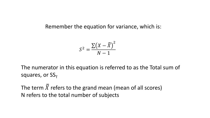
Remember the equation for variance, which is: 2 ?2= ? ? ? 1 The numerator in this equation is referred to as the Total sum of squares, or SST The term ? refers to the grand mean (mean of all scores) N refers to the total number of subjects
The concept behind ANOVA involves partitioning the total sum of squares into component parts. In the case of a 1-way ANOVA, there are two component parts: A within-group sum of squares (SSw), and A between-group sum of squares (SSB) The total sum of squares equals SSw + SSB
Group 1 Group 2 Group 3 ?1 ?2 ? ?3 2, ? ??? ? = ? ? ????? ???? ???= ? ? There are a total of N-1 degrees of freedom. For the chart above, df = 15-1 = 14
Example: Calculation of Total Variance ? = ? 150 15= 10 a1 16 18 10 12 19 a2 4 6 8 10 2 a3 2 10 9 13 11 = ? 2 ? ? ? 1 ??? ? 1= ?2= ?2= ? 102 15 1 ??? ? 1= 380 14 = 27.14 ?2=
Group 1 Group 2 Group 3 ?1 ?2 ? ?3 ? ? 2,? ??? ? = # ?? ???????? ?? ??? ?????,? = # ?? ?????? ??? ?? ???= ?=1 ?=1 Since each group has n-1 degrees of freedom, the total degrees of freedom associated With the SSW is k(n-1), or 3(5-1) = 12
Example: Calculation of Within Groups SS, or SSW ? ? ? ?? 16 18 10 12 19 15 ?? 4 6 8 10 2 6 ?? 2 10 9 13 11 9 ?? ?? ?? ?? ?? ?? 49 1 9 4 0 4 16 16 1 0 16 4 25 9 16 ? ? ?2 60 40 70 ? ? 2= 60 + 40 + 70 = 170 ??? ?? ???= ?=1 ?=1
Group 1 Group 2 Group 3 ?1 ?2 ? ?3 ? 2 ? ?? ? ???= ?=1 Since there are k groups, the total degrees of freedom associated With the SSB is k-1, or 3-1 = 2
Example: Calculation of Between Groups SS, or SSB ? = ? 150 15= 10 = ? ? ?? 16 18 10 12 19 15 25 ?? 4 6 8 10 2 6 16 ?? 2 10 9 13 11 9 1 2 ? ?? ? ???= ?=1 ? ? 2 ? ?? ? ???= ? ?2 ?=1 ???= 5 *(25 + 16 + 1) = 210
Variance is calculated by dividing the sum of squares by the degrees of freedom (n-1). In a similar manner, the Mean Squares Within (MSW) and the Mean Squares Between (MSB) are calculated by dividing the respective sums of squares by the degrees of freedom. Consequently, ???=??? ??? ? 1 ???=??? ??? = = ??? ??? ?(? 1) ???=??? 210 3 1 ??? ???= 170 3(5 1) = 14.17 ???= = = 105 ???
If the numbers were randomly assigned to each group, the expected ratio of MSB/MSW (referred to as the F-ratio) would be around 1.00. This is because we would expect the variance within each group to be similar to the variance between each group. Any systematic change to the values within a group that creates a larger difference between group means (perhaps resulting from a treatment) would increase the magnitude of MSB, while the magnitude of MSW would remain relatively unchanged. Consequently, as the difference between group means increased, so would MSB , along with the resulting F-ratio. When the F-ratio grows to a magnitude that occurs by chance less than 5% of the time, it is considered to be significant, which indicates that there s likely a systematic difference between group means. It does not indicate whether two group means are different, or whether all group means are different, only that a difference exists.
Example: Calculation of F-Ratio From our numeric example, the calculation of the F-ratio would be as follows: F-ratio = MSB / MSW = 105 / 14.17 = 7.41 The degrees of freedom would be: (dfb , dfw), or (2 , 12) The critical F-value associated with these degrees of freedom is 2.8068. Since our calculated F-ratio exceeds the critical F-ratio, we would conclude that at least one of the groups was significantly different from one or more of the other groups. We would then need to run a post-hoc test on the data to find the exact location of the significant difference(s).
Assumptions associated with ANOVA: 1. Within-group variances are normally distributed (detected by Kolomogorov- Smirnov test) 2. Within-group variances are homogenous (detected by Levene s statistic) 3. Between-group observations should be independent 4. Dependent variables should be interval or rational If assumption #1 is not met (indicated by a significant Kolomogorov-Smirnov test), then use Brown-Forsythe F or Welch s F
When more than 2 groups are included in the ANOVA and a significant F-ratio is calculated, use a post-hoc test to determine where significant differences exist. Post-hoc tests enable you to compare all means while holding experiment-wise error constant. The most commonly used post-hoc tests in order of relative stringence are: 1. Scheffe 2. Tukey 3. Bonferroni 4. Newman-Keuls 5. Duncan 6. LSD