Variation of Parameters in Solving Linear Differential Equations
Explore the method of variation of parameters to find particular solutions for linear differential equations, even with non-constant coefficients and general forms of the forcing function. Understand how to approach second-order linear DEs and associated homogeneous equations, with step-by-step processes outlined. Dive into the standard form, determinants, and solution assumptions to enhance your understanding of solving DEs.

Download Presentation

Please find below an Image/Link to download the presentation.
The content on the website is provided AS IS for your information and personal use only. It may not be sold, licensed, or shared on other websites without obtaining consent from the author. If you encounter any issues during the download, it is possible that the publisher has removed the file from their server.
You are allowed to download the files provided on this website for personal or commercial use, subject to the condition that they are used lawfully. All files are the property of their respective owners.
The content on the website is provided AS IS for your information and personal use only. It may not be sold, licensed, or shared on other websites without obtaining consent from the author.
E N D
Presentation Transcript
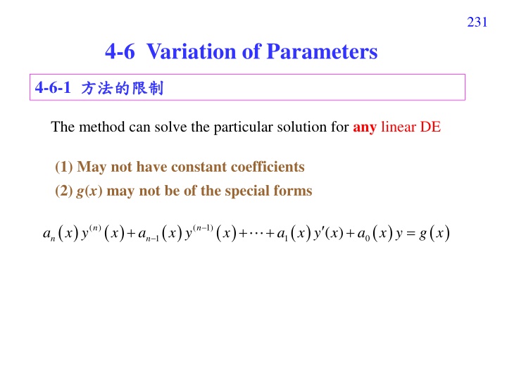
231 4-6 Variation of Parameters 4-6-1 The method can solve the particular solution for any linear DE (1) May not have constant coefficients (2) g(x) may not be of the special forms ( ) x y ( ) x ( ) x y ( ) x ( ) ( ) x y ( ) ( ) + + + + = ( ) n ( 1) n a a a x y x a g x 1 1 0 n n
232 4-6-2 Case of the 2ndorder linear DE ( ) x y x ( ) ( ) x y ( ) ( ) ( ) + + = a a x y x a g x 2 1 0 ( ) x y x ( ) ( ) x y ( ) ( ) + + = associated homogeneous equation: 0 n a a x y x a 1 0 Suppose that the solution of the associated homogeneous equation is + ( ) ( ) 1 1 c y x c y x 2 2 Then the particular solution is assumed as: = + ( ) ( ) u x y x ( ) ( ) p y u x y x 1 1 2 2 ( )
233 = + ( ) ( ) u x y x ( ) ( ) p y u x y x 1 1 2 2 2 = + + + p y 1 1 u y 1 1 u y 2 u y u y u y 2 2 2 1 1 2 2 2 = + + + + + 2 p y 1 1 u y 1 1 u y u y u y u y 2 2 2 ( ) (standard form) ( ) ( ) f x ( ) ( ) + + = y x P x y x Q x y ( ) ( ) ( ) ( ) ( ) ( ) a x a x a x a x g x a x ( ) ( ) ( ) f x = = = , , P x Q x 0 1 2 2 2 ( ) ( ) p p 2 2 + 2 + + = + + + + + 2 2 y P x y Q x y 1 1 u y P u y + 1 1 u y u y + 1 1 u y u y + u y + u y u y 2 2 2 p ( ) ( ) 1 1 2 2 + u y Q u y u y 1 1 2 2 1 1 2 2 zero zero P yu ( ) ( ) p p 1 1 2 2 + + = + + + + + + + y P x y Q x y u y Py Qy + u y Py Qy 1 1 yu 1 u y 1 2 2 p 2 + + + 2 2 2 2 y u u y y u 1 1 2 2 1 1 2
234 ( ) ( ) ( ), f x p p = + + + = p y 1 1 u y u y y P x y Q x y 2 2 p yu ( ) ( ) p p 1 1 u y 2 2 2 + + = + + + + + 2 2 y P x y Q x y y u u y P yu y u 1 1 2 2 1 1 2 p 1 1 u y 2 2 + + + 1 1 yu y u u y 2 2 d dx ( ) f x 2 2 1 1 yu 2 + + + + + = 1 1 yu y u P yu y u y u 2 1 1 2 2 + = 0 1 1 yu ( ) f x 2 2 y u 1 1 y u 2 + = y u 2 + + = = 0 1 1 1 yu yu 2 2 y u y u 0 y y y y u u = 1 2 ( ) f x ( ) f x 1 1 2 2 1 2 2
235 ( ) y f x W W W ( ) = 1 u u x dx 1 = = 2 u 1 + + = = 0 1 1 yu yu 2 2 y u y u 1 ( ) f x ( ) ( ) x dx = 2 y f x W W W 1 1 2 2 u u 2 = = 1 u 2 2 0 ( ) f x 0 ( ) f x y y y y y y y y 1 2 2 1 = = = where W W W 1 2 1 2 2 1 | |: determinant ( ) x ( ) ( ) ( ) x y ( ) x = + p y u x y x u 1 1 2 2 1storder case (page 63)
236 4-6-3 Process for the 2ndOrder Case Step 2-1 standard form y x ( ) ( ) ( ) f x ( ) ( ) + + = P x y x Q x y Step 2-2 0 ( ) f x 0 ( ) f x y y y y y y y y 1 2 2 1 = = = W W W 1 2 1 2 2 1 W W W W 1 = 2 = u u 1 2 Step 2-3 ( ) ( ) x dx = = Step 2-4 1 2 u u x dx u u 1 2 ( ) x ( ) ( ) ( ) x y ( ) x = + Step 2-5 p y u x y x u 1 1 2 2
237 4-6-4 Examples Example 1 (text page 162) + = + 2 x 4 4 ( 1) y y y x e + = 4 4 0: Step 1: solution of y y y = + 2 2 x x cy = ce c xe 1 2 + = = 2 2 x x 2, , y 1 1 u y u y y e y x e Step 2-2: 2 1 2 p 2 2 x x e xe 2 x 0 1) xe = = 4 x W e = = + 4 x ( 1) W x xe + 2 2 2 x x x 2 2 e xe e 1 + + 2 2 2 x x x ( 2 x e xe e 2 x 0 1) e = = + 4 x ( 1) W x e 2 + 2 2 x x 2 ( e x e W W W W 1 = 2 = Step 2-3: = + = 2 1 u x u x x 2 1
238 1 3 + + 1 2 c 1 Step 2-4: = = = + 2 3 2 ( ) u u dx x x dx x x c 1 1 1 2 2 = = + = 2 ( 1) u u dx x dx x x 2 2 1 3 1 2 1 2 1 6 1 2 Step 2-5: = + + = + 3 2 2 2 2 3 2 2 x x x ( ) ( ) ( ) y x x e x x xe x x e p 1 6 1 2 = + + + 2 2 3 2 2 x x x ( ) y ce c xe x x e Step 3: 1 2
239 + = 4 36 csc3 y y x Example 2 (text page 163) + = x c + = cos3 sin3 4 36 0: cy c x y y Step 1: solution of 1 2 + = = ( ) f x csc3 / 4 x 9 csc3 / 4 Step 2-1: standard form: y y x Step 2-2: 0 sin3 x cos3 3sin3 sin3 3cos3 x x = = 3 W = = 1/ 4 W 1csc3 4 x x 1 3cos3 x x cos3 0 x cos3 4 sin3 x x 1 = = W 1 4 2 sin3 csc3 x x W W W W cos3 x x 1 1 1 = 2 = = = u u 1 2 Step 2-3: 12 12 sin3 x u = 1ln sin3 36 Step 2-4: = u x 12 1 2 1 cos3 xdx x ( ) 12 sin3
240 x 1 = + cos3 sin3 ln sin3 x y x x Step 2-5: 12 36 p x 1 Step 3: = + = + + cos3 sin3 cos3 sin3 ln sin3 x y y y c x c x x x 12 36 1 2 c p Note: Interval (0, /6) (0, /3)
241 = 1/ y y x Example 3 (text page 164) = c e + x x cy ce = ( ) 1/ f x x 1 2 x x e e e = = 2 W x x e xedx Note: analytic x t edt t x ( page 49) x 0
242 4-6-5 Case of the Higher Order Linear DE ( ) ( ) ( ) 1 n n a x y x a x y + ( ) x ( ) ( ) x y ( ) ( ) + + + = ( ) n ( 1) n a x y x a g x 1 0 Solution of the associated homogeneous equation: = + + + + ( ) ( ) ( ) ( ) y 1 1 c y x c y x c y x c y x 2 2 3 3 c n n The particular solution is assumed as: = + + + + ( ) ( ) u x y x ( ) ( ) ( ) ( ) ( ) ( ) y u x y x u x y x u x y x 1 1 2 2 3 3 p n n W W = k ( ) ( ) k u x u x dx = ( ) u x k k
243 Process of the Higher Order Case Step 2-1 standard form ( ) ( ) x ( ) ( ) x ( ) ( ) x ( ) ( ) x a x a x a a a x g x a ( ) x ( ) x ( ) + + + + = ( ) n ( 1) n 1 1 0 n y y y x y a n n n n Step 2-2 Calculate W, W1, W2, ., Wn(see page 244) W W W W W W 1 = 2 = n = Step 2-3 u u u 1 2 n Step 2-4 . ( ) 1 1 u u x dx ( ) x dx ( ) x dx = = = 2 n u u u u 2 n ( ) x ( ) ( ) ( ) x y ( ) x ( ) x y ( ) x = + + + y u x y x u u Step 2-5 1 1 2 2 p n n
244 y y y y y y y y y y y y 1 2 3 n W W k = ( ) u x k 1 2 3 n = W 1 2 3 n ( 1) ( 2 1) ( 3 1) ( n 1) n n n n y y y y 1 0 0 y y y y y y y y y y + 1 2 1 1 k k n + 1 2 1 1 k k n = W k ( 2) ( 2 ( 2 ( ) f x 2) ( k 2) ( k 2) ( n 2) n n n n + n 0 ( ) f x y y y y y y y y y y 1 1 1 ( 1) 1) ( k 1) ( k 1) ( n 1) n n n n + n 1 1 1 ( ) ( ) x = / g x a n
245 0 0 ( ) ( ) x Wk: replace the kthcolumn of W by g x a ( ) f x = n 0 ( ) f x For example, when n = 3, y y y y y y y y y 1 2 3 = W 1 2 3 1 2 3 0 0 ( ) f x 0 0 ( ) f x 0 0 ( ) f x y y y y y y y y y y y y y y y y y y 2 3 1 3 1 2 = = = W W W 1 2 3 2 1 3 3 1 2 2 3 1 3 1 2
246 + = 4 sec2 y y x Exercise 30 = + x c + Complementary function: cos2 sin2 cy c c x 1 2 3 1 0 0 cos2 2sin2 4cos2 sin2 2cos2 4sin2 x x = = 8 W x x x x 0 0 cos2 2sin2 4cos2 sin2 2cos2 4sin2 x x = = 2sec2 W x x x x x 1 sec2 x 1 0 0 cos2 2sin2 4cos2 0 0 x 1 0 0 0 0 sin2 2cos2 4sin2 x = = = = 2tan2 W x x x 2 W x x 3 2 sec2 x sec2 x
247 1 W W sec2 tan2 4 W W W W x x 2 = = 1 = 3 = = = u 2 u u 3 1 4 4 1ln cos2 8 x 1ln sec2 8 = = u x u = + tan2 u x x 3 2 1 4 ( ) 1 ln sec2 8 = + + cos2 sin2 x y x c c x c x 1 2 3 1 8 ( ) + + + + tan2 cos2 ln cos2 sin2 x x x x x 4 for - /4 < x < /4 Note: - /4 , /4 are singular points
248 4-6-7 (1) associated homogeneous equation (2) (3) | | determinant (4) u1 (x) u2 (x) (5) f(x) = g(x)/an(x) ( 1storder standard form) (6) u1'(x) u2'(x) + c particular solution yp yp (7) an(x) = 0
249 4-7 Cauchy-Euler Equation 4-7-1 ( ) x ( ) x ( ) ( ) + + + + = ( ) n 1 ( 1) n n n a x y a x y a xy x a y g x 1 1 0 n n k not constant coefficients k ka x but the coefficients of y(k)(x) have the form of akis some constant associated homogeneous equation particular solution ( ) ( ) ( ) x + + ( ) n 1 ( 1) n n n a x y + x a x y 1 n n + = 0 a xy x a y 1 0
250 4-7-2 Associated homogeneous equation of the Cauchy-Euler equation ( ) ( ) 1 n n a x y x a x y x + ( ) + + + = ( ) n 1 ( 1) n n n 0 a xy x a y 1 0 Guess the solution as y(x) = xm, then ( ) m n m n + + n ( 1)( 2) 1 n a a x m m m x ( ) ) m n + m n + + + + 1 1 n ( 1)( 2) 2 x m m m x 1 n ( m n + 2 2 n ( 1)( 2) 3 a x m m m m n x 2 n + + 1 m a x m x = 1 m 0 a x 0
251 Delete xmon the previous page ( ) m n + ( 1)( 2) 1 a m m + + m n ( ( ) ) m n + + ( ( 1)( 1)( 2) 2) 2 3 a m m m 1 n auxiliary function a m m m m n 2 n : constant coefficient + + a m a 1 = 0 0 ! m ( ) ( ) k d dx = m k + 1 1 m m k x ( )! m k k
252 4-7-3 For the 2ndOrder Case ( ) x ( ) + + = 2 0 a x y a xy x a y 2 1 0 auxiliary function: a m m ( ) ( ) + + = 1 0 + + = a m a 2 0 a m a a m a 2 1 0 2 1 2 0 roots ( ) 2 + 4 a a a a a a ( ) 2 4 a a a a a a = 2 1 1 2 2 2 0 m = 2 1 1 2 2 2 0 m 1 a 2 a 2 2 [Case 1]: m1 m2and m1, m2are real two independent solution of the homogeneous part: m m and x x 1 2 = + m m cy c x c x 1 2 1 2
253 [Case 2]: m1= m2 Use the method of reduction of order m y x = 1 1 a 1 dx ( ) P x dx a x e e 2 ( ) x ( ) = = m y y x dx x dx 1 ( ) x 2 1 2 2 1 m y x 1 a a a ( ) x ( ) + + = ( ) 0, y y x y 0 1 Note 1: = P x 1 2 a x a x a x 2 2 2 a a = = m m 2 2 1 Note 2: 1 2 a 2
254 a a a a a 1 1 ln dx x 1 a a a x x x e e 2 2 ( ) x = 2 m = = = 2 2 1 m m m y x dx x dx x dx 1 1 1 1 2 a 2 2 2 m m m x x 1 1 1 2 a a a a 1 1 2 a a ( ) 1 = = = 1 m a m m 1 l n x x x dx x x dx x x 1 2 2 1 1 2 If y2(x) is a solution of a homogeneous DE then c y2(x) is also a solution of the homogeneous DE = m ln y x x If we constrain that x > 0, then 1 2 = + m m ln cy c x c x x 1 1 1 2
255 [Case 3]: m1 m2and m1, m2are the form of m j = + = m j 1 2 two independent solution of the homogeneous part: + j j and C x + x x x + = j j cy C x 1 2 j + + + = = = = ( )ln ln ln lnx j j x x j x ( ) e e e e ( ) + sin( ln ) cos( ln ) x x j x ( ) = cos( ln ) ) ln x sin( ln ) j x x ( ) x j x ( ) = + + ( ) [( )cos ( )sin ln ] cy x C C ( j C C x 1 2 1 2 = + [ cos x c ln sin ln ] cy x c x 1 2
256 Example 1 (text page 167) ( ) x ( ) 4 xy x = 2 2 0 x y y Example 2 (text page 168) ( ) x ( ) + + = 2 4 8 0 x y xy x y
257 Example 3 (text page 169) 1 2 ( ) 1 ( ) 1 y = = 1 y ( ) x + = 2 4 17 0 x y y
258 4-7-4 For the Higher Order Case Process: auxiliary function Step 1-1 roots n independent solutions Step 1-2 solution of the nthorder associated homogeneous equation Step 1-3
259 (1) auxiliary function m0 0 m x associated homogeneous equation (2) auxiliary function m0 k ln , , x x x x m m m m 2 1 k (ln ) , , (ln ) x x x 0 0 0 0 associated homogeneous equation
260 (3) auxiliary function + j j ( ) ( ) ( , cos ln sin x x x ) ln x associated homogeneous equation (4) auxiliary function + j j k ( ) ( ) ( ( ) sin ln (ln ) x x x ( ) ( ) ( ) 2 cos ln , cos ln ln , cos ln (ln ) , , x x x x x x x x 1 k cos ln (ln ) x x x ) ( ) 2 sin ln , sin ln ln , sin ln (ln ) , , x x x x x x x x 1 k associated homogeneous equation 2k
261 Example 4 (text page 169) ( ) x y ( ) x ( ) 8 xy x + + + = 3 2 5 7 0 x x y y auxiliary function ( )( ) ( ) + + + = 1 2 5 1 7 8 0 m m m m m m + + + + = 3 2 2 3 2 5 5 7 8 0 m m m m m m + + + = 3 2 2 4 8 0 m m m )( ) ( + + = 2 2 4 0 m m
262 4-7-5 Nonhomogeneous Case To solve the nonhomogeneous Cauchy-Euler equation: Method 1: (See Example 5) (1) Find the complementary function (general solutions of the associated homogeneous equation) from the rules on pages 252-255, 259-260. (2) Use the method in Sec. 4-6 (Variation of Parameters) to find the particular solution. (3) Solution = complementary function + particular solution Method 2: See Example 6 Set x = et, t = ln x
263 Example 5 (text page 169, illustration for method 1) ( ) 3 x y x xy x ( ) 3 + = 2 4 x 2 y x e Step 1 solution of the associated homogeneous equation auxiliary function ( ) 1 m m m = 1 + = 2 4 3 0 m m + = 3 3 0 m 1 m = 3 = c x c x + 3 2 cy 1 2 3 x x x = = Step 2-2 Particular solution 3 2 W x 2 1 3 0 x 3 0 x x = = 3 x = = 2 W x e 5 x 2 W x e 2 2 x 1 1 2 x e 2 2 x 2 3 x e W W W W 1 = 2 = Step 2-3 = = 2 x x u e u x e 2 1
264 1 = = + 2 x x x 2 2 u u dx x e xe e Step 2-4 1 2 = = x u u dx e 2 = + = 2 x x 2 2 p y 1 1 u y u y x e xe Step 2-5 2 2 Step 3 = c x c x + + 3 2 x x 2 2 y x e xe 1 2
265 Example 6 (text page 170, illustration for method 2) ( ) ( ) x y x xy x + = 2 ln y x Set x = et, t = ln x (Step 1) 1 x dt dy dx dt dy dx dt dy = = (chain rule) 2 1 x dt x dt = 1 d y dx d dx dx d y dy dt d dx dt dx d dy d dy = = = 2 2 2 1 x dt 1 x dt x 1 1 x dy dt d y dt dy dt = + 2 2 2 2 Therefore, the original equation is changed into 2 d dt d dt ( ) + = 2 ( ) y t ( ) y t y t t 2 (Step 2) This process can be simplified using the auxiliary function.
266 2 d dt d dt ( ) + = 2 ( ) y t ( ) y t y t t 2 (Step 3) = + + + t t ( ) y t 2 ce c te t 1 2 = c x c x + + + ( ) y x ln ln 2 ( t = ln x ) x x 1 2 (Step 4) Note 1: d dt k d y dx ( ) ( ) means D = + k 1 1 x D k D D y t t t t k (Step 2) (Step 2) Determine the auxiliary function, then replace m by Dt Note 2: : Cauchy-Euler equation auxiliary function
267 4-7-6 (1) Section 4-3 ex x x ln(x) auxiliary function mn (2) particular solution? Variation of Parameters ( ) m n + ( 1)( 2) 1 m m m (3) x = 0 (Why?)
268 Extra Problems: How do we solve ( ) ( ) + = 0 xy x y x (1) ( ) + = 2 ( 1) ( ) y x 0 x y x (2)
269 linear DE (1) numerical approach (Section 4-9-3) (2) using special function (Chap. 6) (3) Laplace transform and Fourier transform (Chaps. 7, 11, 14) (4) (table lookup)
270 (1) Section 4-7 DE (2) linear DE constant coefficient linear DE
271 Exercises for practicing Section 4-6 4, 5, 8, 13, 14, 17, 18, 21, 25, 28, 29, 34 Section 4-7 11, 17, 18, 20, 21, 24, 32, 35, 36, 37, 40, 42 Review 4 27, 28, 29, 30, 32, 42


