Wave Propagation in Solid-Fluid Layered System Analysis
wave propagation in a solid-fluid layered system, this study dives into frequency-dependent slowness surfaces, caustics, dispersion analysis, and more. Detailed diagrams and matrices illustrate the dynamics of waves in different layers.

Download Presentation

Please find below an Image/Link to download the presentation.
The content on the website is provided AS IS for your information and personal use only. It may not be sold, licensed, or shared on other websites without obtaining consent from the author.If you encounter any issues during the download, it is possible that the publisher has removed the file from their server.
You are allowed to download the files provided on this website for personal or commercial use, subject to the condition that they are used lawfully. All files are the property of their respective owners.
The content on the website is provided AS IS for your information and personal use only. It may not be sold, licensed, or shared on other websites without obtaining consent from the author.
E N D
Presentation Transcript
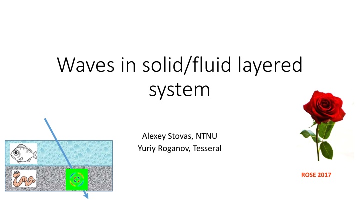
Waves in solid/fluid layered system Alexey Stovas, NTNU Yuriy Roganov, Tesseral ROSE 2017
Outline Wave propagation in solid-fluid layers Frequency dependent slowness surface From phase to group domain Caustics Dispersion Analysis Conclusions
Solid-fluid layers 1 1 1 = = = 2 2 2 : , , Slowness surfaces in individual layers q p q p q p f 2 2 2 f = v Ea : Solid ( ) T ( ) T = = d P d S u P u S a v , , , , , , , A A A A u u 1 3 13 33 p q p q q q p p = E ( ) ( ) 1 2 1 2 2 2 2 2 2 2 2 2 pq p pq p ( ) ( ) 1 2 1 2 2 2 3 2 2 3 2 2 p pq p pq = w E b : Fluid f ( ) T ( ) T = = d S u S b w , , , B B u 3 33 q q f f f f = E f f f f f
Solid-fluid layers Let us consider the diagonal matrices and propagator matrices ( ) i q H 1 exp 0 0 0 2 ( ) i q H 1 0 exp 0 0 2 = , ( ) i q H 1 0 0 exp 0 2 ( ) i q H 1 0 0 0 exp 2 i q H f exp 0 2 = f i q H f 0 exp = = 1 P Q E E E E ( ) solid 2 1 ( ) fluid f f f
Periodic fluid-solid system Fluid z1 z2 ( ) ( ) ( ) z w ( ) ( ) ( ) z = = = w Qw z z 2 1 v Pv z z Solid z3 4 2 Qw z4 z5 5 4 Fluid z
Monodromy matrix : At the boundaries between liquid and solid layers and are continuous and Fv Gw ( w v ) ( ) z ( ) z = = 0 w Mw 3 = = 33 13 5 1 , , M = QFPGQ where 0 0 1 0 0 0 0 1 2 12 21 r r i = F 1 11 12 r r 21 22 r r + 11 12 r r r r 21 22 r r r r f M = P P P P 11 22 r r 32 31 34 31 11 12 21 22 2 1 i f 1 0 0 0 0 1 11 12 r r 21 22 r r = G ( ) i qH is an eigenvalue of matrix M exp Similar approach is proposed by Schoenberg, 1983; 1984
Frequency dependent slowness surface = 11 12 r r r r Hq 2 tan 2 21 22 2 H 11 12 r r r r ( ) = , arctan q p 21 22
f = 100 Hz Slowness surface : Horizontal velocities A F E r C H = , : 0 12 r = = = : : 0 0 0 22 11 r r E : =0.001 f = 10 Hz 21 H : Model = = 4.0 2.2 1.5 = km s km s km s Slow S*-wave D B f = 1000 Hz G Fast S*-wave f = 3 2.7 1.0 = = g cm g cm P-wave 3 f A C F 0.001 H km ( ) ,2011 Korneev
Group velocity surface: fluid effect at f=10Hz = 0.1 = 0.5 = 0.001
Group domain G : Caustics + B 21 22 11 r r 12 r r r r r r D = + D 11 12 21 22 G A C E H F D G
Horizontal velocity dispersion H=1m : Horizontal velocities P wave A r Fast S wave V E r F V min ( ) = , 0 is weakly dispesive S V 12 max S V min ( ( ) = F , 0 is weakly dispesive max 22 ) = F , 0 V C r is dispesive H=10m min 11 Slow S wave V F V min ( ( ) ) = S , 0 F r is weakly dispesive max 12 S V = S , 0 V H r is dispesive max min 21 S V min
P wave vertical velocity ( ) ( ) 1 1 fH fH fH fH + + tan tan tan tan 1 1 fH f f = arctan ( ) f ( ) ( ) v 1 1 fH fH fH fH 0 P tan tan 1 tan tan f f = f f f Backus 0 1 1 ( ) ( ) = + + 1 ( ) 0 f 2 P 2 2 f v 0
Analysis (large p and large frequency*) ( ) 1 1 1 max , , If p f ( ) ( ( ) x i tan tanh ix i ) ( ) ix = lim tan x Sq q Sq q iS q iS q f f = = = = , , , 11 r 12 r r r 21 22 q q ( ) 2 f = + 1 2 + 2 4 2 2 4 S p q q p f : Solutions q i S = ( ) = non Scholte wave propagating wave 0 ( )
Analysis (zero frequency) 0 f ( ) p ( ) p 2 f 2 q q 1 p v ( ) ( ) p ( ) ( ) = + + 2 1 1 q ( ) f 2 2 PL 1 f = 0.1 2 ( ) = 2 1 = v Lamb wave velocity 0.01 PL 2 = 0.001 Generally, it is different from Backus, however, gives similar results for small .
Analysis: zero limit (inherited slip) ( ( 1 2 ) ) ( ( ) ) ( ( ) ) 2 ( ( ) ) 1 2 + 2 2 2 4 tan 4 tan p fHq p q q fHq 1 fH ( ) ( ) = lim tan tan q fHq fHq 2 0 + 2 2 2 4 tan 4 tan p fHq p q q fHq ( ) a homogeneous anisotropic layer with the slip at both interfaces + + + + + 2 2 2 2 ( ) = lim 30 q f Hz 0 2 2 2 1 1 p ( ) ij c = = lim , q 0 2 0 0 1 4 2 2 1 p f 2 0 0 lim q A homogeneous anisotropic medium with the slip smeared within the whole medium 0 0 f . 2 2 = = : 0 2 1 Anisotropic parameters and 2 2 ( ) sameresultcanbeobtained fromBackus
Stop bands for vertically propagated P wave ( ) + 1 fH 1 1 R R fH f f = tan tan 0 = 0.1 0 f = 0.2 = 0.3 Pass Pass Stop Stop
Fluid substitution (Utsira sand, f=30Hz) CO2 Water 1. Vp0&eps are weakly dependent on frequency; 2. Anisotropic parameter is strong negative and frequency dependent. d=1cm CO2 Water d=5cm
Conclusions The frequency-dependent slowness surface is defined for waves propagating in a solid-fluid system (periodical). It consists of three sheets corresponding to P- and two S-waves. Both S*-waves have triplications. The low- and high-frequency limits are defined. The frequency dispersion is computed for horizontally propagating S-waves. The stop-bands for P-wave are defined. When the fluid layer thickness tends to zero, we obtain the medium with inhereted slip. It is shown that S-waves are sensitive to fluid substitution.


")
")
")

")