Wireless Radio Channel Propagation Models

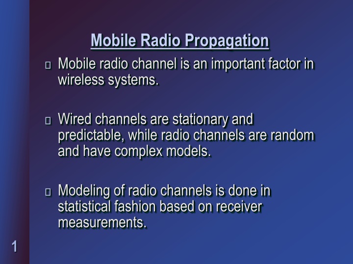
Mobile Radio Propagation Mobile radio channel is an important factor in wireless systems. Wired channels are stationary and predictable, while radio channels are random and have complex models. Modeling of radio channels is done in statistical fashion based on receiver measurements. 1

Types of propagation models Large scale propagation models To predict the average signal strength at a given distance from the transmitter Controlled by signal decay with distance Small scale or fading models. To predict the signal strength at close distance to a particular location Controlled by multipath and Doppler effects. 2

Radio signal pattern -30 Received Power (dBm) -40 -50 -60 -70 14 16 18 20 22 24 26 28 T-R Separation (meters) 3

Measured signal parameters Electrical Field (Volts/m) Magnitude E = IEI Vector Direction E = xEx + yEy + zEz Power (Watts or dBm) Power is scalar quantity and easier to measure. 4

Relation between Watts and dBm P (dBm) = 10 log10 [P(mW)] P(mW) P(dBm) 10 10 1 0 10-1 -10 10-2 -20 10-6 -60 5

Physical propagation models Free Space Propagation Transmitter/receiver have clear LOS (Line Of Sight) path Reflection Wave reaches receiver after reflection off surfaces larger than wavelength Diffraction Wave reaches receiver by bending at sharp edges (peaks) or curved surfaces (earth). Scattering Wave reaches receiver after bouncing off objects smaller than wavelength (snow, rain) 6

Free Space Propagation Transmitter and receiver have clear, unobstructed LOS path between them. (Courtesy: webbroadband.blogspot.com) 7

LOS (Friis) transmission equation Pr = Pt Gt Gr 2 (4 )2 d2 L Pt = Transmitted Power (W) Pr = Received Power (W) Gt = Transmitter antenna gain Gr = Receiver antenna gain L = System loss factor Due to line losses, but not due to propagation L 1 8

Antenna Gain Power Gain of antenna G = 4 Ae / 2, Ae is effective aperture area of antenna Wavelength = c / f (Hz) = 3 108 / f , meters 9

Example A transmitter produces 50W of power. If this power is applied to a unity gain antenna with 900 MHz carrier frequency, find the received power at a LOS distance of 100 m from the antenna. What is the received power at 10 km? Assume unity gain for the receiver antenna. 10

Solution Pr = Pt Gt Gr 2 (4 )2 d2 L Pt = 50 W, Gt = 1, Gr = 1, L = 1, d = 100 m = (3 108) / (900 106) = 0.33 m Solving, Pr= 3.5 10-6 W Pr (10 km) = Pr(100 m) (100/10000)2 = 3.5 10-6 (1/100)2 = 3.5 10-10 W 11

Electric Properties of Material Bodies Fundamental constants Permittivity = 0 r , Farads/m Permeability = 0 r ,Henries/m Conductivity , Siemens/m Types of materials Dielectrics allow EM waves to pass Conductors block EM waves Metamaterials bend EM waves 12

Ground Reflection (2-Ray Model) T (transmitter) Pr = PLOS +Pref PLOS Pi R (receiver) ht Pref hr d 13

Ground Reflection Equations For d > 20hthr / , Received power Pr= 2 2 P G G h h t t r t r 4 d 14

Example A mobile is located 5 km away from a base station, and uses a vertical /4 monopole antenna with a gain of 2.55dB. Assuming carrier frequency of 900 MHz and transmitted power of 100 W with 10 dB antenna gain, find the received power at the mobile using the 2-ray model if the height of the transmitting antenna is 50 m and receiving antenna is 1.5 m above the ground. 15

Solution T (transmitter) Pr = PLOS +Pref PLOS Pi R (receiver) 50 Pref 1.5 d 16

Gain of receiving antenna = 2.55 dB => 1.8 Gain of transmitting antenna = 10 dB => 10 Received power Pr= 2 2 P G G h h t t r t r 4 d = 100 10 1.8 502 1.52 (5 103)4 = 0.0162 W 17

Diffraction Diffraction allows radio signals to propagate around the curved surface or propagate behind obstructions. (Courtesy: electronics-notes.com) 18

Knife-edge Diffraction Geometry T h h R d1 d2 ht hr 19

Diffraction Parameter and Gain Diffraction parameter + 2 ( ) d d v = 1 d 2 h d 1 2 Diffracted power = LOS power+ Diffraction Gain Pd = PLOS + Gd(dB) 20

Empirical formula for Gain v Gd (dB) v -1 -1 v 0 0 v 1 1 v 2.4 20 log (0.4 [0.1184 (0.38 0.1 v)2] v 2.4 20 log (0.225 / v) 0 20 log (0.5 0.62 v) 20 log (0.5 e-0.95v ) 21

Example Compute the diffraction power at the receiver assuming: Transmitter frequency = 900 MHz LOS received power = 50 mW d1 = 1km d2 = 1km h = 25m 22

Solution Diffraction parameter v = (3 108) / (900 106) = 0.33 m = + 2 ( ) d d 1 d 2 h d 1 2 + 2 1000 ( 1000 ) = 2.74 => v = 25 ( 0 1000 )( 3 . 1000 )( ) Using the table, Gd (dB) = 20 log (0.225/2.74) = -22 dB Hence diffracted power Pd = PLOS + Gd (dB) = 10 log(50) -22 = -5.01 dBm => 0.316 mW 23

Scattering When a radio wave impinges on a rough surface, the reflected energy is spread out in all directions Examples of scattering surfaces: lamp posts, trees, cars, rain, snow. (Courtesy:http://www.tpub.com/) 24

Radar Cross Section (RCS) Model RCS (Radar Cross Section) = Power density of scattered wave in direction of receiver Power density of radio wave incident on the scattering object 25

Scattering Power Equation PR = PT GT 2 RCS (4 )3 dT 2 dR 2 PT = Transmitted Power GT = Gain of Transmitting antenna dT = Distance of scattering object from Transmitter dR = Distance of scattering object from Receiver 26

Practical Propagation models Most radio propagation models are derived using a combination of analytical and empirical models. Empirical approach is based on fitting curves or analytical expressions that recreate a set of measured data. 27

Pros and cons of empirical models Takes into account all propagation factors, both known and unknown. Disadvantages: New models need to be measured for different environment or frequency. 28

Path Loss (PL) Model Transmitter receiver model T d0 R PT PR(d0) PR(d) Logarithmic model ( dB) PL(d) = PL(d0) + 10n log10 (d/d0) Received power( dBm) PR(d) = Pt PL(d) 29

Emprical values of path loss factor n Environment n Free space Urban area cellular radio LOS in building 2 2.7 3.5 1.6 1.8 30

More accurate propagation models Logarithmic path loss normal gives only the average value of path loss. Surrounding environment may be vastly different at two locations having the same T R separation d. More accurate model includes a random variable with standard deviation to account for change in environment. 31

Practical propagation model development Values of n and are computed from measured data. Linear regression method which minimizes the difference between measured and estimated path Estimated over a wide range of measurement locations and T R separations. 32

Random Propagation Model equation Probability [ PR (d) > ] = (d ) P R Q Probability [ PR (d) < ] = (d ) P R Q Average received power is calculated using logarithmic model (d ) PR 33

2 2 / / 2 2 z z e e ( ( ) ) ~ ~ Q Q z z 2 z 2 z Calculation of Q Function e x2/2 e x x 2 x 1 2 z z Q(z) = Q function = dx 2 Q(z) table from Appendix F of book (Rappaport), for z values 0 < z < 3.9 For z > 3.9, use the approximation: 2 / 2 z e ( ) ~ Q z 2 z 34

Q Function Table 35

Example Four received power measurements were taken at the distances of 100m, 200m, 1 km and 3 km from a transmitter. T-R distance 100 m 0 dBm 200 m 1 km 3 km Measured Power - 20 dBm - 35 dBm - 70 dBm 36

Example a. Find the minimum mean square error (MMSE) estimate for the path loss exponent n, assuming d0 = 100m. b. Calculate the standard deviation about the mean value. c. Estimate the received power at d = 2 km using the resulting model. d. Predict the likelihood that the received signal at 2 km will be greater than 60 dBm. 37

Solution Let Pi be the average received power at distance di : Pi (d) = P (d0) 10n log (d/100) d = d0 = 100m = Pi (d0) = P0= 0 dBm 38

a. d1= 200 m, P1= -3n, d2= 1 km, P3= -10n, d3= 3 km, P4= -14.77n Mean square error J = (P Pi)2 = (0 0)2 + [-20 (-3n)]2 + [-35 (-10n)]2 + [-70 (-14.77n)]2 = 6525 2887.8n + 327.153n2 Minimum value = > dJ(n) / dn = 654.306n 2887.8 = 0 n = 4.4 39

b. Variance 2 = J / 4 = ( P Pi)2 / 4 = (0+0) + (-20+13.2)2 + (-35+44)2 + (-70+64.988)2 4 = 152.36 / 4 = 38.09 = 6.17 dB 40

c. Pi (d = 2 km) = 0 10(4.4) log (2000/100) = -57.24 dBm 41

d. Probability that the received signal will be greater than 60 dBm is: PR = [PR(d) > -60 dBm] = Q [( - PR (d)) / ] = Q [(-60 + 57.24) / 6.17] = Q [- 0.4473] = 1 Q [0.4473] = 1 0.326 = 0.674 = > 67.4% _____ 42

Percentage of Coverage Area Given a circular coverage area of radius R In the area A, the received power PR The area A is defined as U( ) R r Area A 43

Calculation of Coverage Area U( ) Use Figure 4.18 from book (Rappaport) 44

Example For the previous problem, predict the percentage of area with a 2 km radius cell that receives signals greater than 60 dBm. 45

Solution From solution to previous example, Prob [PR (R) > ] = 0.674 =>( / n) = 6.17 / 4.4 = 1.402 From table 4.18, Fraction of total area = 0.92 => 92% 46

Outdoor Propagation Models Longley Rice model point-to-point communication systems (40MHz 100MHz) Okumara s model widely used in urban areas (150 MHz 300 MHz) Hata model graphical path loss (150 MHz 1500 MHz) 47

Indoor Propagation Models Log-distance path loss model Ericsson multiple breakdown model 48