Methods for Extending Streamflow Records and Their Importance
The presentation outlines methods for extending streamflow records, the reasons behind doing so, and the process of using the results. It includes examples of using data from long-term sites to estimate records at short-term sites. The importance of extending records is highlighted, emphasizing the potential impact on frequency curves due to missing flows in short records. Various techniques, including linear regression, are discussed to bridge gaps in streamflow data, ensuring a comprehensive analysis and understanding of water resource dynamics.

Methods for Extending Streamflow Records and Their Importance
PowerPoint presentation about 'Methods for Extending Streamflow Records and Their Importance'. This presentation describes the topic on The presentation outlines methods for extending streamflow records, the reasons behind doing so, and the process of using the results. It includes examples of using data from long-term sites to estimate records at short-term sites. The importance of extending records is highlighted, emphasizing the potential impact on frequency curves due to missing flows in short records. Various techniques, including linear regression, are discussed to bridge gaps in streamflow data, ensuring a comprehensive analysis and understanding of water resource dynamics.. Download this presentation absolutely free.
Presentation Transcript
Methods for Extending Streamflow Records Beth Faber, PhD, PE USACE, HEC Chuck Parrett, PH Ryan Cahill retired, USGS Hydrologist USACE, NWP
Back in the USGS days Chuck P 2 2
Outline of Presentation Streamflow Record Extension what is it ? why would we do it ? some methods for doing it how do we use the result ? Brief Review of Linear Regression 3
Extending Streamflow Records Using data from a similar long-term site to estimate data (extend the record) at a short-term site USGS 11266500 USGS 11268200 MERCED R. NR BRICEBURG, CA MERCED R. AT POHONO BRIDGE NR YOSEMITE, CA 25000 25000 Annual Peak Streamflow (cfs) Annual Peak Streamflow (cfs) 20000 20000 15000 15000 10000 10000 5000 5000 0 0 1910 1930 1950 1970 1990 2010 1964 1966 1968 1970 1972 1974 1976 4
Merced River sites long record site short record site 5
Extending Streamflow Records Using data from a similar long-term site to estimate data (extend the record) at a short-term site USGS 11266500 USGS 11268200 USGS 11268200 MERCED R. NR BRICEBURG, CA MERCED R. NR BRICEBURG, CA MERCED R. AT POHONO BRIDGE NR YOSEMITE, CA 25000 25000 25000 Annual Peak Streamflow (cfs) Annual Peak Streamflow (cfs) Annual Peak Streamflow (cfs) 20000 20000 20000 15000 15000 15000 10000 10000 10000 5000 5000 5000 0 0 0 1910 1930 1950 1970 1990 2010 1964 1910 1966 1930 1968 1950 1970 1990 2010 1970 1972 1974 1976 6
Why Should We Extend a Record? A short record may be missing large recorded flows that could have a significant effect on a frequency curve USGS 11266500 USGS 11268200 MERCED R. NR BRICEBURG, CA MERCED R. AT POHONO BRIDGE NR YOSEMITE, CA 25000 25000 Annual Peak Streamflow (cfs) Annual Peak Streamflow (cfs) 20000 20000 15000 15000 10000 10000 5000 5000 0 0 1910 1930 1950 1970 1990 2010 1910 1930 1950 1970 1990 2010 7 7
Extending Streamflow Record --Another View... Long Record Site Short Record Site 1960 1962 1964 1966 1968 1970 1972 1974 1976 1978 1980 1982 1984 1986 1988 1990 1992 1994 1996 1998 2000 Use the relationship to fill- in missing record at the short-term site (N2=13) Year Develop a relationship from the concurrent record (N1=18) 8 8
Basic Linear Regression Concept Can knowing the value of one variable help predict the value of another variable? 120 We try to find the best linear equation that relates one variable to another. Hydrologic data often have linear relationships if we use logs 100 80 Variable Y 60 40 20 0 0 5 10 15 20 25 30 Variable X 9 9
Basic Linear Regression Concept If there is no relationship, the best prediction of variable Y is simply the mean of Y 120 120 error 100 100 this estimate would include some error 80 80 Variable Y Variable Y 60 60 40 40 20 20 0 0 0 0 5 5 10 10 15 15 20 20 25 25 30 30 Variable X Variable X 10
Basic Linear Regression Concept If variable X has some ability to help predict variable Y, we seek a relationship between the two 120 120 error 100 100 this estimate also has some error 80 80 Variable Y Variable Y 60 60 40 40 20 20 0 0 0 0 5 5 10 10 15 15 20 20 25 25 30 30 Variable X Variable X 11
Ordinary Least-Squares (OLS) Regression The best linear relationship between variable X and variable Y is one that minimizes the sum of squared errors 120 error Y = m X + b m = slope b = intercept the metrics R2 and standard error tell the quality of the regression 100 80 Variable Y 60 40 20 0 0 5 10 15 20 25 30 12 Variable X 12
Basic Linear Regression Assumptions Both X and Y are random variables with no measurement error There s a linear relationship between X and Y (or some transformation of X and/or Y) Regression errors are independent homoscedastic i.e., evenly distributed across X Normally distributed 13 13
Measures of Regression Quality R2 = coefficient of determination, squared correlation, % of the variability in Y explained by the variability in X 14 14
Linear Correlation correlation = 0 correlation = 0.7 correlation = 1.0 correlation = -0.6 correlation = -1.0 15
Measures of Regression Quality R2 = coefficient of determination, squared correlation % of the variability in Y explained by the variability in X Standard error (SE) = square root of the sum of squared errors Do not rely solely on R2 and SE to judge regression quality! 16 16
Regression Diagnostics Plot the data! Same line, R2, and SE on all graphs! (Anscombe 1973) and same everything else 17 17
Record Extension Developing and Using the Relationship Step 1: Develop a linear relationship between X and Y (the long and short record stations) using the concurrent record N1 = concurrent Step 2: Use the linear relationship to estimate values for the short record station for times we only have values for the long record station (non-concurrent!) N2 = only long 18
40000 X12 etowah Y1 suwanee n1 Annual Maximum Streamflow (cfs) 35000 30000 25000 20000 15000 10000 5000 0 1940 1880 1900 1920 1960 1980 2000 2020 N1 = concurrent record, N2 = additional record X12 etowah Y2 suwanee n2 Y1 suwanee n1 40000 Annual Maximum Streamflow (cfs) 35000 30000 25000 20000 15000 10000 5000 0 1940 1880 1900 1920 1960 1980 2000 2020 19
Statistics (based on logs) for Concurrent Record (N1) longer record station shorter record station ?? ?? ? ? ? ? ?? ?? ?? ?? ?=? ?=? ?? ?? ? ? (?? ?)? (?? ?)? ? ? ?? ?? ? ?? ?? ? ?=? ?=? r 20
Ordinary Least Squares (OLS) Regression Basic equation for record extension using statistics from concurrent record Estimate each point in the non-concurrent period, Yi, based on the longer record value, Xi, and the concurrent statistics. ??= ? + ??? ?? ? ?? X = Longer station Y = Shorter station 21 21
OLS Regression Assuming the linear model is valid, and that X is measured without error, OLS yields predictions that are: Unbiased Minimum variance OLS is the preferred method of predicting a particular value of Y, given a value of X But, if our purpose is NOT the best single prediction, but rather the description of a relationship between X and Y, then OLS is not appropriate. 22
OLS Regression But, if our purpose is NOT the best single prediction, but rather the description of a relationship between X and Y, then OLS is not appropriate. If |r| < 1 (nonperfect fit), then variance of predicted values of Y will tend to be less than variance of true values. That is, ?< ?? ? ? ? ? Reduced variance for a series of estimates is a major problem for record extension to be used for frequency analysis 23 23
Reduction in Variance variance of estimates is reduced Estimates of variable Y, when only variable X is available, will follow the regression line 120 120 100 100 80 80 Variable Y Variable Y 60 60 40 40 20 20 Concurrent Record, N1 Extended Record, N2 0 0 0 5 10 15 20 25 30 0 5 10 15 20 25 30 Variable X Variable X 24
Other Methods that Do Not Reduce Variance Other methods for developing Linear Regressions that do not reduce variance of predictions OLS Regression Plus Noise (RPN) Other linear regressions generally termed Maintenance Of Variance Extension (MOVE) methods MOVE.1 and MOVE.2 described by Hirsch, and MOVE.3 described by Vogel and Stedinger (1985) Two-station comparison used in Bulletin 17B (MOVE.2) 25
RPN (OLS Regression Plus Noise) Matalas and Jacobs address the problem of biased (reduced) variance by adding some random noise to the regression equation. ??= ? + ??? ?? ? + ? ?? ?? ?? ?? ei = standard normal random variable, N[0, 1] ?2(?1 4)(?1 1) (?2 1)(?1 3)(?1 2) = 26
RPN (OLS Regression Plus Noise) As noted by Matalas and Jacobs, RPN is not too appealing. Independent studies of the same sequence of x and y by several investigators lead to different values of [the mean, standard deviation, and estimated values of y] because the same sequence of pseudo-random numbers is unlikely to be used 27 27
MOVE.1 Maintenance of Variance Extension (MOVE) Method 1 was described by Hirsch (1982). The equation is only slightly different from the OLS equation: No r term here ?? ?? X = Longer station Y = Shorter station ??= ? + ?? ? Nearly unbiased variance of estimates 28 28
Line of Organic Correlation (LOC) (Alternatively called MOVE.1) The LOC is the line that minimizes the sum of squared geometric distances in both the X and Y directions This method does not reduce variance of predictions Minimize areas of right triangles 29 29
OLS vs MOVE.1 (LOC) For streamflow record extension applications, LOC produces higher estimates for large flows and lower estimates for small flows r = 0.93 30
MOVE.2 The MOVE.2 method described by Hirsch (1982) ALSO uses information from the long-term record, outside the concurrent record, to define the relationship Not just X1, but also X2, to define the line Hirsch found that MOVE.2 variance is essentially unbiased But, equations for estimating missing record are a bit hairy Chuck P 31
MOVE.2 Line ????? ????? X = Longer station Y = Shorter station ??= ????+ ?? ???? ???? ??? ?? ????= ??+ ?? ?? ??+ ?? Matalas-Jacobs Estimators ? ?????= ? + ? + ? ??+ ?? ? 32 N1 = concurrent record, N2 = additional record 32
MOVE.2 Line ? X = Longer station Y = Shorter station ?????= ? + ? + ? ??+ ?? ? N1 = concurrent record N2 = additional record ? ? = (?? ?)??? ? ???? ? = (?? ?) ????? ?+ (?? ?) ? (? ??)??? ? ??? ? ?( ?? ??)? ???? (??+??) ????? ? = ??? 33
MOVE.3 The MOVE.3 method described by Vogel and Stedinger (1985) also uses information from the long-term record X (Matalas-Jacobs estimators), and in a way that assures that the complete extended record for Y will have a mean and variance matching the Matalas-Jacobs MJ estimators. Vogel and Stedinger determined that MOVE.3 variance is unbiased. But, equations for estimating missing record are even hairier than for MOVE.2 . Chuck P 34 34
MOVE.3 Line X = Longer station Y = Shorter station ?? = ? + ?(?? ??) N1 = concurrent record, N2 = additional record ???? ?? ?? ?? ??+ ?? ? = ??+ ?? ? ? ??( ?? (?? ?)??? ????)? ??(? ????) ? ????? (?? ?)??? ??= ? 35 35
But, dont forget. Linear equations and statistics for all methods are based on Bi-Variate Normal distributions of random Independent Data. Real-world flow data probably are skewed (even when using logs) Real-world data may have some serial correlation 36 36
Record Extension For Flood Frequency Bulletin 17B, Appendix 7 Two-station comparison: used the Matalas-Jacobs estimators (MOVE.2) to adjust the mean and varianceof a short record frequency curve, based on correlation with a long record Bulletin 17C, Appendix 8 Use MOVE.3 to extend the short record, and perform frequency analysis Why? PILFs and historical data, regional skew, etc But, the uncertainty will be too small! We don t really have N = N1+N2 Should extend only a portion of the available long record, ne 37 37
MOVE.3 (Bulletin 17C version) Original MOVE.3 allows for extension based on every additional (non- concurrent) value of the long-term site (N2) False sense of confidence in frequency estimates at the short-term site So, extend only a portion of the long-term site s years Define ne = equivalent record length, and the maximum number of years allowable for extension. Higher correlation = higher ne for r = 1, ne = N2 Modify MOVE.3 equations for a and b to use ne instead of N2 ne N2 N1
Which ne years to extend? Only ne years of record extension are recommended Which years should we pick? Different year selections . will not affect the MJ mean or variance, but will affect the skew Bulletin 17C allows for judgment of the analyst on year selection to ensure the skew isn t misrepresented Ne? Ne? Ne? Ne? 39
Which ne years to extend? 17C Default: use the most recent years But if a sequence of unusually big floods or small floods is in ne, may need to adjust: 1. Compute the skew using a record extension for the entire period of record (original MOVE.3 technique using N2, not limited to ne) 2. Select a sequence of ne years that results in a similar skew value 3. HEC-SSP has an option to do this Ne? Ne? Ne? Ne? 40
How Should We Select a Long-Term Site for Record Extension? Various studies have recommended that the correlation coefficient (r) between short-term and long-term sites for the concurrent record be 0.8 or greater. Long-term sites with non-concurrent flows that are substantially outside the range in the concurrent period may provide more information than other potential long-term sites. Can use more than one long-term site and weight results (perhaps using r or record length) with results from another long-term site. In general, use long-term sites in close proximity to the short- term site, with a reasonable duration of overlap. 41
Record Extension Method Comparison For many real- world datasets, the various record extension techniques produce similar regression lines 42
Take-Home Message(s) From Me Chuck P For record extension, MOVE.1 is simple, easy to apply, and likely to be as good as MOVE.2 or MOVE.3 for real-world data The record extension method (MOVE.3) described in the new Bulletin 17C should be used for flood-frequency applications It has official sanction It has statistical guidelines for applicability and a measure for Ne 43 43
Sidebar: Drainage Area Ratio Uses a ratio of the drainage area between two locations to estimate periods of missing flow. ?? ?? ? = ? Y = flow estimate at missing station X = known flow at long-term station Ay = Drainage area of missing station Ax = Drainage area of long-term station = 1, unless there is a regional regression study Missing station (downstream): Drainage Area = 270 sq. miles Long-term station (upstream): Drainage Area = 211 sq. miles DAR = 270/211 = 1.28 44
Sidebar: Drainage Area Ratio Generally works well when two sites are on the same river, with drainage areas within 50% of each other Can produce poor results if different streams are used. Always use a record extension technique (e.g. MOVE.3) instead of a drainage area ratio when concurrent record is available. 45
Summary of Estimation Techniques Method Purpose Uses Drainage Area Ratio Approximate analysis is good enough Two gages are very close together, minimal effort Ordinary Least Squares (OLS) Regression Best individual flow estimates Someone wants to get the best estimate peak flow for one particular year Maintenance of Variance Extension (MOVE.1) Filling in daily flows in an extended period Water resources planning and management models; reservoir design and operation Maintenance of Variance Extension (MOVE.3, Bulletin 17C) Estimate flood peaks for years with missing data Flood-Frequency Analysis 46
References Alley, W. M., and A. W. Burns, 1983. Mixed-station extension of monthly streamflow records, J. Hydraul. Div. Am. Soc. Civ. Eng., 109(10), p. 1271-1284. Bulletin 17B, 1982. Guidelines for Determining Flow Frequency Analysis: Interagency Advisory Committee on Water Data, USGS, Office of Water Data Collection, Reston, Virginia. England, J.F. Jr., Cohn, T.A., Faber, B.A., Stedinger, J.R., Thomas, W.O., Jr., Veilleux, A.G., Kiang, J.E., and Mason, R.R., Jr., 2018, Guidelines for determining flood flow frequency Bulletin 17C: U.S. Geological Survey Techniques and Methods, book 4, chap. B5, 148 p https://doi.org/10.3133/tm4B5. 47 47
References Helsel, D.R., and Hirsch, R.M., 2002, Statistical methods in water resources: Techniques of Water-Resources Investigations of the U.S. Geological Survey, Book 4, Chapter A3. , New York, Elsevier, 510 p. https://pubs.usgs.gov/twri/twri4a3/pdf/twri4a3-new.pdf Hirsch, R.M., 1982, A comparison of four streamflow record extension techniques: Water Resources Research, v. 18, no. 4, p. 1081-1088. Matalas, N.C. and Jacobs, B., 1964, A correlation procedure for augmenting hydrologic data: U.S. Geological Survey Professional Paper 434-E. Vogel, R.M., and Stedinger, J.R., 1985. Minimum Variance Streamflow Record Augmentation Procedures: Water Resources Research V21(5), p715-723. 48 48


 Regression")


 for Concurrent")
 Regression")


")
")

")
")


")


 From Me…")