Introduction to Three-Level Meta-Analysis Models in R: A Practical Example

Explore three-level meta-analysis models in R with a focus on the association between paternal anxiety and child emotional problems. Learn to prepare data files, fit models using the rma.mv function in metafor, and understand the structure of the formula for random effects. Follow along with a step-by-step guide using R-Studio for analysis.

Introduction to Three-Level Meta-Analysis Models in R: A Practical Example
PowerPoint presentation about 'Introduction to Three-Level Meta-Analysis Models in R: A Practical Example'. This presentation describes the topic on Explore three-level meta-analysis models in R with a focus on the association between paternal anxiety and child emotional problems. Learn to prepare data files, fit models using the rma.mv function in metafor, and understand the structure of the formula for random effects. Follow along with a step-by-step guide using R-Studio for analysis.. Download this presentation absolutely free.
Presentation Transcript
An Introduction to Three-Level Meta- Analysis Models in R A practical example using R Francesca Zecchinato
A three-level meta-analysis looking at the association between paternal anxiety and child emotional problems
Preparing the data file - prepare a .csv file Nested random-effects model: individual effect sizes (level 2) nested within samples (level 3)
Schematic representation of the data Aggregated cluster effects pooled in a three- level meta-analysis Samples used in primary studies Results of individual participants pooled in primary studies from Harrer et al., 2021 (https://bookdown.org/MathiasHarrer/Doing_Meta_Analysis_in_R/multilevel-ma.html)
In R-Studio - install or call the packages - import the data file (named anxietydataset.csv )
In R-Studio - once imported in R, we can use the head() function to see the general structure of the data
Model fitting A three-level meta-analysis model can be fitted in R using the rma.mv function in {metafor}. Here is a list of the most important arguments for this function, and how they should be specified: yi. The name of the column in our dataset which contains the calculated effect sizes. (It is recommended to transform r to Fisher-z transformed correlations, which have better mathematical properties than untransformed correlations.). In our case, it is column fisher_z. V. The variance of the calculated effect sizes. In our case, this is var_z. slab. The name of the column in our dataset which contains the study labels. data. The name of the dataset. test. The test we want to apply for our regression coefficients; "t , which uses a test similar to the Knapp- Hartung method, is recommended. method. The method used to estimate the model parameters. "REML"(restricted maximum-likelihood) is usually recommended.
Model fitting random. In this argument, we specify a formula which defines the (nested) random effects. In our example, individual effect sizes (level 2) are nested within samples (level 3). How do we specify this in our rma.mv function? We use a slash (/) to separate the higher- and lower-level grouping variable. To the left of /, we put in the level 3 (cluster) variable. To the right, we insert the lower-order variable nested in the larger cluster. The general structure of the formula looks like this: ~ 1 | cluster/effects_within_cluster. In our example, we assume that individual effect sizes (level 2; defined by es_r_id) are nested within samples (level 3; defined by sample_id). This results in the following formula: ~ 1 | sample_id/es_r_id.
Running the model The complete rma.mv function looks like this:
Running the model Random-effects variances calculated for each level of our model. Sigma^2.1 shows the level 3 between- cluster variance. Sigma^2.2 shows the variance within clusters (level 2). In the nlvls column, we see the number of groups on each level. Level 3 has 27 groups, equal to the K= 27 included samples. These 27 samples contain 116 effect sizes, as shown in the second row.
Running the model Model results Under Model Results, we see the estimate of our pooled effect, which is z= 0.15 (95%CI: 0.10 0.20). To facilitate the interpretation, it is advisable to transform the effect back to a normal correlation. This can be done using the convert_z2r function in the {esc} package:
How do I present the findings? Summary table
How do I present the findings? Summary table Written summary Offspring emotional outcomes were drawn from 27 samples (116 effect sizes, 33 individual studies) and were positively associated with paternal anxiety, r = 0.15 (95% CI [.10, .20]; p < .0001). I2 was 86.02%, with estimated variance components 2Level 3= 0.01 and 2Level 2= 0.01, meaning that I2Level 3= 52.42% of the total variation could be attributed to between-cluster, and I2Level 2= 33.6% to within-cluster heterogeneity.
Recommended further reading and resources Viechtbauer W. Conducting meta-analyses in R with the metafor package. Journal of statistical software 2010; 36(3): 1-48. Harrer M, Cuijpers P, Furukawa TA, Ebert DD. Doing Meta-Analysis With R: A Hands-On Guide. 1st ed. Boca Raton, FL and London: Chapman & Hall/CRC Press; 2021.


")