Approximating Binomial Distribution with Normal Distribution

Teachings for Exercise 3F

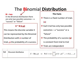
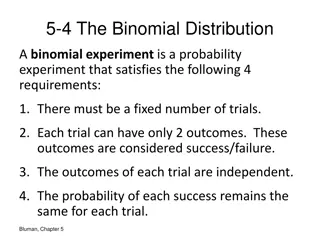
? =? ? ? The normal distribution You need to be able to approximate a binomial distribution Let s compare the two quickly Normal distribution Continuous data Binomial distribution Discrete data No. heads when flipping a coin 7 times Height of the flipped coin You can use the processes you have learnt for the normal distribution to approximate a binomial distribution under 2 conditions The value of ?(the number of trials) must be large (this will mean the distribution is smoother) The probability of success must be close to 0.5 (if it is not, then the distribution will not be symmetrical) 3F

? =? ? Using normal distribution to approximate a binomial distribution ? must be large ? must be close to 0.5 ? The normal distribution ? = ?? You need to be able to approximate a binomial distribution Let ?~?(100,0.45) So ? is binomially distributed, we are doing 100 trials with a 0.45 chance of success on each trial Starting with a Binomial distribution, ?~?(?,?) Therefore, we would expect that on average, we get 100 0.45 = 45 successes We are going to use a normal distribution to approximate it (for example, the binomial distribution tables you are given only go up to ? = 50 So the mean is the product of ? and ? Therefore, ? = ?? Finding a relationship for the standard deviation is much more difficult to understand So we are going to use a normal distribution ?~?(?,?) We will need to clarify some statements first We need to be able to get from ? and ? to the values of ? and ? 3F

?~?(?,?) ?~?(?,?) ? = ?? The normal distribution ? 1 2 3 4 5 6 ? 10 10 10 10 10 10 ?? 10 20 30 40 50 60 You need to be able to approximate a binomial distribution The expected value of a set of data is essentially its mean. Imagine we had a normal unbiased 6 sided dice. If we rolled it 60 times we would expect to get 10 of each number. ?? = 210 ? = 60 Mean = ?? ? Sub in values Let ? be the number we get when rolling the dice, ? be the frequency of that number, and ? be the total number of trials Mean = 210 60 Calculate Mean = 3.5 3F

?~?(?,?) ?~?(?,?) ? = ?? The normal distribution ? ?(?) ? ?(?) You need to be able to approximate a binomial distribution 1 16 16 16 16 16 16 16 26 36 46 56 66 2 The expected value of a set of data is essentially its mean. 3 4 5 However, rather than doing a trial and using that to calculate the mean (ie its expected value), you can calculate it using the probabilities of each event happening 6 ? ?(?)=21 6 ? ?(?)= 3.5 Doing this calculates the expected value straight away, without needing to divide by ? 3F

?~?(?,?) ?~?(?,?) ? = ?? The normal distribution You need to be able to approximate a binomial distribution What you have just seen is showing that the following two calculations are equivalent ? ? ? ?(?) = Multiply each outcome by its probability, and then add them all up after Add all the outcomes up, and divide by how many there are in total (note that in the example we used ??, but the idea is the same add up all the values! The fx just sped things up a bit) So really it is (? ?(?)) 3F

? ? ?~?(?,?) ?~?(?,?) ? = ?? ? ?(?) = The normal distribution ?2 1 4 9 16 25 36 ??2 10 40 90 160 250 360 ? 1 2 3 4 5 6 ? 10 10 10 10 10 10 You need to be able to approximate a binomial distribution It does not matter what set of values we start with. For example, if the starting values were all ?2 instead of ? ??2= 910 ? = 60 Mean of ?2 = ??2 ? Sub in values Mean of ?2 = 910 60 Calculate Mean of ?2 = 15.16 So the expected value of ?2is 15.16 3F

? ? ?~?(?,?) ?~?(?,?) ? = ?? ? ?(?) = The normal distribution ?2 ?2 ?(?) ? ?(?) You need to be able to approximate a binomial distribution 1 1 16 16 16 16 16 16 16 46 96 166 256 366 2 4 It does not matter what set of values we start with. 3 9 4 16 5 25 Like the previous example, we can find the expected value of ?2 by using the original probabilities 6 36 ?2 ?(?)=91 6 ?2 ? ?= 15.16 3F

?2 ? ? ? ?~?(?,?) ?~?(?,?) ? = ?? ?2 ?(?) ? ?(?) = = The normal distribution You need to be able to approximate a binomial distribution What you have just seen is showing that the following two calculations are equivalent ?2 ? ?2 ?(?) = Multiply each squared outcome by its probability, and then add them all up after Add all the squared outcomes up, and divide by how many there are in total So really it is (?2 ?(?)) 3F

?2 ? ? ? ?~?(?,?) ?~?(?,?) ? = ?? ?2 ?(?) ? ?(?) = = The normal distribution 2 ?2= ?2 You need to be able to approximate a binomial distribution ? ? The second part of this is the mean squared ? Remember that we already have an expression for the mean from before! ?2= ?2 Can you remember the formula for the variance of a data set from year 12? ??2 ? What we need to do now is to find a way to replace the first part in terms of ? and ?, the number of trials and the probability of success in the binomial distribution So we need to focus on rewriting this part We can replace the first part using the equivalent calculation that we saw before (?2 ?(?)) ?2= ?2 ??2 ? Replace first term using the above ?2= (?2 ?(?)) ??2 3F

?~?(?,?) ?~?(?,?) ? = ?? The normal distribution Imagine we are considering the number of heads when tossing a biased coin 5 times. Let ? = ?????? ?? ????, and ? ???? = 0.4 You need to be able to approximate a binomial distribution Lets put together a table Can you remember the formula for the variance of a data set from year 12? ?2 ?(?) 02 5 0 12 5 1 22 5 2 32 5 3 42 5 4 52 5 5 ? ?(?) 5 0 5 1 5 2 5 3 5 4 5 5 0.400.65 0.400.65 0 So we need to focus on rewriting this part 0.410.64 0.410.64 1 (?2 ?(?)) 0.420.63 0.420.63 2 ? 0.430.62 0.430.62 3 Remember how to find the calculation for a an event that is binomially distributed? ? ???1 ?? ? ?2 = 0.440.61 0.440.61 4 ?=0 0.450.60 0.450.60 5 ? ? (We will be summing the values ??1 ?? ? ? ? = ? = from ? = 0 up to ? = ?????? ?? ?????? ) ? ???1 ?? ? ?2 So we are doing this calculation for each value of ?, and then adding them up 3F

? ???1 ?? ? ?~?(?,?) ?~?(?,?) ? = ?? ? ? = ? = The normal distribution You need to be able to approximate a binomial distribution You hopefully also remember the following from year 12 (Binomial expansion powerpoint) ?! ? ? = Can you remember the formula for the variance of a data set from year 12? ? ? !?! So now we need to rewrite this ? ? ???1 ?? ? ?2 = Replace the first bracket using the relationship shown ?=0 ? ?! ?2 ? ? !?!??1 ?? ? = Group together ?=0 ? ?2 ?!??1 ?? ? ? ? !?! = ?=0 3F

? ???1 ?? ? ?~?(?,?) ?~?(?,?) ? = ?? ? ? = ? = The normal distribution ? ?2 ?!??1 ?? ? ? ? !?! You need to be able to approximate a binomial distribution The first term will be when ? = 0 ?=0 This first term will therefore be 0, due to the ?2 part, so we do not need to include it in the summation Can you remember the formula for the variance of a data set from year 12? ? ?2 ?!??1 ?? ? ? ? !?! Therefore, we can start the summation from ? = 1 instead ?=1 So now we need to rewrite this ? ?2 ?!??1 ?? ? ? ? !?! This term is 1 2 3 ..(? 1) ? = ?=0 We can cancel one of the first ?2 terms with the ? from this factorial So this term would now become ? 1 ! ? ? ?!??1 ?? ? ? ? !(? 1)! = ?=1 3F

? ???1 ?? ? ?~?(?,?) ?~?(?,?) ? = ?? ? ? = ? = The normal distribution Remember that this is a summation of a number of terms ? ? ?!??1 ?? ? ? ? !(? 1)! You need to be able to approximate a binomial distribution = ?=1 The number of terms (?) and the probability (?) are a constant Can you remember the formula for the variance of a data set from year 12? ? This means we can factorise them outside of the summation ? (? 1)!?? 11 ?? ? ? ? !(? 1)! = ?? ?=1 So now we need to rewrite this The ?! term has been changed as in the previous example ? ?2 ?!??1 ?? ? ? ? !?! = The ?term has been adjusted as well ?=0 It is important to note that we cannot factorise the ? term outside. This is because in the summation, for the first term ? = 1, for the second term ? = 2, and so on Since ? takes different values, we cannot factorise it out as would then multiply everything by only a single value 3F

? ???1 ?? ? ?~?(?,?) ?~?(?,?) ? = ?? ? ? = ? = The normal distribution Let ? = ? 1 So ? = ? + 1 ? ? (? 1)!?? 11 ?? ? ? ? !(? 1)! You need to be able to approximate a binomial distribution ?? This will affect most terms ?=1 We will now be starting on ? = 0 instead of ? = 1 Can you remember the formula for the variance of a data set from year 12? We have not changed the number of terms though, so the final term will now be ? 1 ? 1 So now we need to rewrite this (? + 1) (? 1)!??1 ?? ? 1 ? ? 1 !(?)! ?? ? ?2 ?!??1 ?? ? ? ? !?! ?=0 = ?=0 3F

? ???1 ?? ? ?~?(?,?) ?~?(?,?) ? = ?? ? ? = ? = The normal distribution You need to be able to approximate a binomial distribution ? 1 (? + 1) (? 1)!??1 ?? ? 1 ? ? 1 !(?)! ?? We can write this as two separate summations (using the ? + 1 ?=0 ? 1 ? 1(? 1)!??1 ?? ? 1 ? ? 1 !(?)! ? (? 1)!??1 ?? ? 1 ? ? 1 !(?)! = ?? + ?=0 ?=0 ?! (? 1)! ? ? 1 !?! ? ? ? 1 ? = = ? ? !?! What if we let ? = ? 1 and ? = ?? ? 1 ? 1 ? 1 ? ? 1 ? ??1 ?? ? 1+ ??1 ?? ? 1 = ?? ? ?=0 ?=0 3F

? ???1 ?? ? ?~?(?,?) ?~?(?,?) ? = ?? ? ? = ? = The normal distribution This term represents all possible outcomes in a trial, so it will always equal 1 regardless of the values chosen for ?, ? and ? You need to be able to approximate a binomial distribution ? 1 ? 1 ? 1 ? ? 1 ? ??1 ?? ? 1+ ??1 ?? ? 1 ?? ? ?=0 ?=0 Lets think about the second summation, using heads on the biased coin from before as an example Let the number of trials, ?, equal 3 Let ?(?????) = 0.4 Remember this is going to be the sum of the terms from ? = 0 to ? = 2 2 2 ?0.4?0.62 ? ?=0 When ? = 0 When ? = 1 When ? = 2 2 1 2 2 2 0 0.410.61 0.420.60 0.400.62 + + What will these add up to? They will add up to 1 as they represent all possible outcomes (from 2 choose 0 + from 2 choose 1 + from 2 choose 2) 3F

? ???1 ?? ? ?~?(?,?) ?~?(?,?) ? = ?? ? ? = ? = The normal distribution You need to be able to approximate a binomial distribution ? 1 ? 1 ? 1 ? ? 1 ? ??1 ?? ? 1+ ??1 ?? ? 1 ?? ? ?=0 ?=0 If ? is the number of heads on a coin, this part represents the probability of each value of ? happening ? 1 ? 1 ? ??1 ?? ? 1+ 1 ?? ? ?=0 ie) We can rewrite this as ?(?) The only difference is that the number of terms is ? 1, which is accounted for in the summation term ? 1 ?? ? ? ? + 1 ?=0 ? ? ??1 ?? ? ? ? = ? = 3F

? ???1 ?? ? ?~?(?,?) ?~?(?,?) ? = ?? ? ? = ? = The normal distribution You need to be able to approximate a binomial distribution ? 1 This term is saying to multiply all the possible values of ? by their probabilities, and then add the answers up ?? ? ? ? + 1 ?=0 What does that give us? It gives us the expected value of ? And how do we calculate the expected value if we know the number of trials and the probability of success? = ?? ? 1 ? + 1 Multiply the number of trials by the probability of success! In this case, the probability of success is ?, and the number of trials is (? 1) So the expected value of ? is ? 1 ? 3F

? ???1 ?? ? ?~?(?,?) ?~?(?,?) ? = ?? ? ? = ? = The normal distribution ? = ??(1 ?) 2 ?2= ?2 You need to be able to approximate a binomial distribution ? ? ? Earlier, we replaced the mean with ?? ?2= ?2 If you remember (quite a while back), we were finding an expression for the variance ??2 Now we can replace the expected value of ?2 with the expression we found ? ?2= ?? ? 1 ? + 1 ??2 Multiply the inner bracket The expression we just found is that: ?2= ?? ?? ? + 1 ??2 Multiply the square bracket ?? ? 1 ? + 1 ?2= ??2 ??2+ ?? ??2 Simplify A reminder that we were finding this so we could use it to replace the expected value of ?2, which we can now do! ?2= ?? ??2 Factorise ?2= ??(1 ?) Square root ? = ??(1 ?) 3F

?~?(?,?) ?~?(?,?) ? = ?? The normal distribution ? = ??(1 ?) You need to be able to approximate a binomial distribution ? = ?? Sub in values ? = (100)(0.53) Calculate A biased coin has ? ???? = 0.53. The coin is tossed 100 times and the number of heads, X, is recorded. ? = 53 ? = ??(1 ?) a) Write down a binomial model for ? ?~?(100,0.53) Sub in values ? = (100)(0.53)(1 0.53) Calculate b) Explain why ? can be approximated using a normal distribution Since ? is large and ? is close to 0.5 ? = 4.99 c) Find the values of ? and ? in this approximation 3F

?~?(?,?) ?~?(?,?) ? = ?? The normal distribution ? = ??(1 ?) You need to be able to approximate a binomial distribution Something to be careful is that the normal distribution is continuous and the binomial distribution is discrete You need to apply a continuity correction The binomial random variable ?~?(150,0.48) is approximated by the normal random variable ?~?(72,6.122). Since ? is the continuous distribution, any values up to 70.5 would round to 70 when converted to the binomial distribution ?(? 70) a) Use this approximation to find ?(? 70) So you need to go up to 70.5 when calculating = ?(? < 70.5) = 0.4032 Use your calculator with ? = 72, ? = 6.12, lower limit of -100 and upper limit of 70.5 = 0.4032 3F

?~?(?,?) ?~?(?,?) ? = ?? The normal distribution ? = ??(1 ?) You need to be able to approximate a binomial distribution Apply the continuity correction ?(80 ? < 90) Be careful! The upper limit should not include 90. As such, in the continuous distribution we should not go higher than 89.5 The binomial random variable ?~?(150,0.48) is approximated by the normal random variable ?~?(72,6.122). = ?(79.5 ? < 89.5) Use your calculator with a lower limit of 79.5, upper limit of 89.5, ? = 72 and ? = 6.12 = 0.1081 a) Use this approximation to find ?(? 70) = 0.4032 b) Also use the approximation to find ?(80 ? < 90) 3F

?~?(?,?) ?~?(?,?) ? = ?? The normal distribution ? = ??(1 ?) You need to be able to approximate a binomial distribution ? ? ??1 ?? ? ? ? = ? = Sub in values, with the number of yellow bulbs being 30 For a particular type of flower bulb, 55% will produce yellow flowers. A random sample of 80 bulbs is planted. 80 50 0.55500.4530 ? ? = 50 = Calculate ? ? = 50 = 0.0365 Calculate the percentage error incurred when using a normal approximation to estimate the probability that there are exactly 50 yellow flowers. ? ? = 50 = 0.0365 First, calculate the actual probability using the binomial distribution 3F

?~?(?,?) ?~?(?,?) ? = ?? The normal distribution ? = ??(1 ?) You need to be able to approximate a binomial distribution ? = ?? Sub in values ? = (80)(0.55) Calculate For a particular type of flower bulb, 55% will produce yellow flowers. A random sample of 80 bulbs is planted. ? = 44 ? = ??(1 ?) Calculate the percentage error incurred when using a normal approximation to estimate the probability that there are exactly 50 yellow flowers. Sub in values ? = (80)(0.55)(1 0.55) Calculate ? = 4.45 ? ? = 50 = 0.0365 Now convert the problem to a normal distribution ? = 4.45 ? = 44 3F

?~?(?,?) ?~?(?,?) ? = ?? The normal distribution ? = ??(1 ?) You need to be able to approximate a binomial distribution ?~?(80,0.55) Convert using the values we calculated ?~?(44,4.452) For a particular type of flower bulb, 55% will produce yellow flowers. A random sample of 80 bulbs is planted. Apply continuity corrections and change to a normal distribution calculation ?(? = 50) Calculate the percentage error incurred when using a normal approximation to estimate the probability that there are exactly 50 yellow flowers. = ?(49.5 < ? < 50.5) Use your calculator with a lower limit of 49.5, upper limit of 50.5, ? = 44 and ? = 4.45 = 0.0362 ? ? = 50 = 0.0365 Now convert the problem to a normal distribution ? = 4.45 ? = 44 3F

?~?(?,?) ?~?(?,?) ? = ?? The normal distribution ? = ??(1 ?) You need to be able to approximate a binomial distribution ? 49.5 < ? < 50.5 = 0.0362 ? ? = 50 = 0.0365 Divide the difference by the correct value For a particular type of flower bulb, 55% will produce yellow flowers. A random sample of 80 bulbs is planted. % ????? =0.0003 0.0365 100 Calculate the percentage error incurred when using a normal approximation to estimate the probability that there are exactly 50 yellow flowers. = 0.82% ? ? = 50 = 0.0365 Now convert the problem to a normal distribution ? = 4.45 ? = 44 3F