DBMS Internals and Query Optimization: Understanding Relational Algebra Equivalences

Database Applications (15-415) DBMS Internals- Part X Lecture 22, April 3, 2018 Mohammad Hammoud

Today Last Session: DBMS Internals- Part IX Query Optimization Today s Session: DBMS Internals- Part X Query Optimization (Cont d) Announcements: Quiz II will be held on Sunday, April 8 (all concepts covered after the midterm are included) PS4 is due on April 11 by midnight Project 3 is due on Sunday, April 15 by midnight

DBMS Layers Queries Query Optimization and Execution Continue Relational Operators Files and Access Methods Transaction Manager Recovery Manager Buffer Management Lock Manager Disk Space Management DB

Relational Algebra Equivalences A relational query optimizer uses relational algebra equivalences to identify many equivalent expressions for a given query Two relational algebra expressions over the same set of input relations are said to be equivalent if they produce the same result on all relations instances Relational algebra equivalences allow us to: Push selections and projections ahead of joins Combine selections and cross-products into joins Choose different join orders

RA Equivalences: Selections Two important equivalences involve selections: 1. Cascading of Selections: ( ) ( ) R ( ) R ... ... 1 1 c cn c cn Allows us to combine several selections into one selection OR: Allows us to replace a selection with several smaller selections 2. Commutation of Selections: ( c 1 ) ( ) ( ) R ( ) R 2 2 1 c c c Allows us to test selection conditions in either order

RA Equivalences: Projections One important equivalence involves projections: Cascading of Projections: ( ) R ( ( ( ) R ) ) ... 1 1 a a an This says that successively eliminating columns from a relation is equivalent to simply eliminating all but the columns retained by the final projection!

RA Equivalences: Cross-Products and Joins Two important equivalences involve cross-products and joins: 1. Commutative Operations: (R S) (S R) (R S) (S R) This allows us to choose which relation to be the inner and which to be the outer!

RA Equivalences: Cross-Products and Joins Two important equivalences involve cross-products and joins: 2. Associative Operations: R (S T) (R S) T R (S T) (R S) T R (S T) (T R) S It follows: This says that regardless of the order in which the relations are considered, the final result is the same! This order-independence is fundamental to how a query optimizer generates alternative query evaluation plans

RA Equivalences: Selections, Projections, Cross Products and Joins Selections with Projections: ( ( )) ( ( )) R R a c c a This says we can commute a selection with a projection if the selection involves only attributes retained by the projection! Selections with Cross-Products: R T ( ) R S c c This says we can combine a selection with a cross-product to form a join (as per the definition of a join)!

RA Equivalences: Selections, Projections, Cross Products and Joins Selections with Cross-Products and with Joins: S R c ) ( S R c ) ( ( ) R S c ( ) R S c Caveat: The attributes mentioned in c must appear only in R and NOT in S This says we can commute a selection with a cross-product or a join if the selection condition involves only attributes of one of the arguments to the cross-product or join!

RA Equivalences: Selections, Projections, Cross Products and Joins Selections with Cross-Products and with Joins (Cont d): ) ( c c c ( 1 c c ( 1 c c ( ) R S R S ( 1 2 3 c ( ))) R S 2 3 c ) ( ( )) R S 2 3 c This says we can push part of the selection condition c ahead of the cross-product! This applies to joins as well!

RA Equivalences: Selections, Projections, Cross Products and Joins Projections with Cross-Products and with Joins: ( 1 a a ) ( a c a ( ) ) ( ) R S R S 2 a ( ) ( ) R S R S c 1 2 a ( ) ( ( ) ( )) R S R S a c a c 1 2 a a Intuitively, we need to retain only those attributes of R and S that are either mentioned in the join condition c or included in the set of attributes a retained by the projection

How to Estimate the Cost of Plans? Now that correctness is ensured, how can the DBMS estimate the costs of various plans? sname sname Canonical form rating > 5 rating > 5 bid=100 sid=sid sid=sid Sailors bid=100 Sailors Reserves Reserves

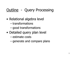
Outline A Brief Primer on Query Optimization Query Evaluation Plans So far Relational Algebra Equivalences Estimating Plan Costs Enumerating Plans Nested Sub-Queries

Estimating the Cost of a Plan The cost of a plan can be estimated by: 1. Estimating the cost of each operation in the plan tree Already covered last week (e.g., costs of various join algorithms) 2. Estimating the size of the result set of each operation in the plan tree The output size and order of a child node affects the cost of its parent node How can we estimate result sizes?

Estimating Result Sizes Consider a query block, QB, of the form: SELECT attribute list FROMR1, R2, ., Rn WHERE term 1 AND ... AND term k What is the maximum number of tuples generated by QB? NTuples (R1) NTuples (R2) . NTuples(Rn) Every term in the WHERE clause, however, eliminates some of the possible resultant tuples A reduction factor can be associated with each term

Estimating Result Sizes (Contd) Consider a query block, QB, of the form: SELECT attribute list FROMR1, R2, ., Rn WHERE term 1 AND ... AND term k The reduction factor (RF) associated with each term reflects the impact of the term in reducing the result size Final (estimated) result cardinality = [NTuples (R1) ... NTuples(Rn)] [ RF(term 1) ... RF(term k)] Implicit assumptions: terms are independent and distribution is uniform! But, how can we compute reduction factors?

Approximating Reduction Factors Reduction factors (RFs) can be approximated using the statistics available in the DBMS s catalog For different forms of terms, RF is computed differently Form 1: Column = Value RF = 1/NKeys(I), if there is an index I on Column Otherwise, RF = 1/10 count E.g., grade = B A F NKeys(I) grade

Approximating Reduction Factors (Contd) For different forms of terms, RF is computed differently Form 2: Column 1 = Column 2 RF = 1/MAX(NKeys(I1), NKeys(I2)), if there are indices I1 and I2 on Column 1 and Column 2, respectively Or: RF = 1/NKeys(I), if there is only 1 index on Column 1 or Column 2 Or: RF = 1/10, if neither Column 1 nor Column 2 has an index Form 3: ColumnIN (List of Values) RF equals to RF of Column = Value (i.e., Form 1) # of elements in the List of Values

Approximating Reduction Factors (Contd) For different forms of terms, RF is computed differently Form 4: Column > Value RF = (High(I) Value)/ (High(I) Low(I)), if there is an index I on Column Otherwise, RF equals to any fraction < 1/2 count E.g., grade >= C A F grade

Improved Statistics: Histograms Estimates can be improved considerably by maintaining more detailed statistics known as histograms Distribution D Uniform Distribution Approximating D 10 10 9 9 8 8 7 7 6 6 5 5 4 4 3 3 2 2 1 1 0 0 1 2 3 4 5 6 7 8 9 10 11 12 13 14 0 0 1 2 3 4 5 6 7 8 9 10 11 12 13 14

Improved Statistics: Histograms Estimates can be improved considerably by maintaining more detailed statistics known as histograms Distribution D What is the result size of term value > 13? 10 9 8 7 6 9 tuples 5 4 3 2 1 0 0 1 2 3 4 5 6 7 8 9 10 11 12 13 14

Improved Statistics: Histograms Estimates can be improved considerably by maintaining more detailed statistics known as histograms Uniform Distribution Approximating DWhat is the (estimated) result size of term value > 13? 10 9 8 7 6 (1/15 45) = 3 tuples 5 4 3 2 Clearly, this is inaccurate! 1 0 0 1 2 3 4 5 6 7 8 9 10 11 12 13 14

Improved Statistics: Histograms We can do better if we divide the range of values into sub-ranges called buckets Equiwidth histogram Equidepth histogram 10 10 9 9 8 8 Uniform distribution per a bucket 7 7 Equal # of tuples per a bucket 6 6 5 5 4 4 3 3 2 2 1 1 0 0 0 1 2 3 4 5 6 7 8 9 10 11 12 13 14 0 1 2 3 4 5 6 7 8 9 10 11 12 13 14 Bucket 1 Count=8 Bucket 2 Count=4 Bucket 3 Count=15 Bucket 4 Count=3 Bucket 5 Count=15 Bucket 1 Count=9 Bucket 2 Count=10 Bucket 3 Count=10 Bucket 4 Count=7 Bucket 5 Count=9

Improved Statistics: Histograms We can do better if we divide the range of values into sub-ranges called buckets Equiwidth histogram What is the (estimated) result size of term value > 13? 10 9 8 Uniform distribution per a bucket The selected range = 1/3 of the range for bucket 5 Bucket 5 represents a total of 15 tuples Estimated size = 1/3 15 = 5 tuples 7 6 5 4 3 2 Better than regular histograms! 1 0 0 1 2 3 4 5 6 7 8 9 10 11 12 13 14 Bucket 1 Count=8 Bucket 2 Count=4 Bucket 3 Count=15 Bucket 4 Count=3 Bucket 5 Count=15

Improved Statistics: Histograms We can do better if we divide the range of values into sub-ranges called buckets Equidepth histogram What is the (estimated) result size of term value > 13? 10 9 8 The selected range = 100% of the range for bucket 5 Bucket 5 represents a total of 9 tuples Estimated size = 1 9 = 9 tuples 7 Equal # of tuples per a bucket 6 5 4 3 2 Better than equiwidth histograms! Why? 1 0 0 1 2 3 4 5 6 7 8 9 10 11 12 13 14 Bucket 1 Count=9 Bucket 2 Count=10 Bucket 3 Count=10 Bucket 4 Count=7 Bucket 5 Count=9

Improved Statistics: Histograms We can do better if we divide the range of values into sub-ranges called buckets Equidepth histogram Because, buckets with very frequently occurring values contain fewer slots; hence, the uniform distribution assumption is applied to a smaller range of values! 10 9 8 7 Equal # of tuples per a bucket 6 5 4 3 What about buckets with mostly infrequent values? They are approximated less accurately! 2 1 0 0 1 2 3 4 5 6 7 8 9 10 11 12 13 14 Bucket 1 Count=9 Bucket 2 Count=10 Bucket 3 Count=10 Bucket 4 Count=7 Bucket 5 Count=9

Outline A Brief Primer on Query Optimization Query Evaluation Plans Relational Algebra Equivalences Estimating Plan Costs Enumerating Plans Nested Sub-Queries

Enumerating Execution Plans A B C D Consider a query Q = Here are 3 plans that are equivalent: D D C C D B A C B A B A Left-Deep Tree Linear Trees A Bushy Tree

Enumerating Execution Plans A B C D Consider a query Q = Here are 3 plans that are equivalent: D D C C D B A C B A B A Why?

Enumerating Execution Plans (Contd) There are two main reasons for concentrating only on left- deep plans: As the number of joins increases, the number of plans increases rapidly; hence, it becomes necessary to prune the space of alternative plans Left-deep trees allow us to generate all fully pipelined plans Clearly, by adding details to left-deep trees (e.g., the join algorithm per each join), several query plans can be obtained The query optimizer enumerates all possible left-deep plans using typically a dynamic programming approach (later), estimates the cost of each plan, and selects the one with the lowest cost!

Enumerating Execution Plans (Contd) In particular, the query optimizer enumerates: 1. All possible left-deep orderings 2. The different possible ways for evaluating each operator 3. The different access paths for each relation Assume the following query Q: SELECT S.sname, B.bname, R.day FROM Sailors S, Reserves R, Boats B WHERE S.sid = R.sid AND R.bid = B.bid

Enumerating Execution Plans (Contd) In particular, the query optimizer enumerates: 1. All possible left-deep orderings x B B R R S S S R B x R S S B S B R R B

Enumerating Execution Plans (Contd) In particular, the query optimizer enumerates: 1. All possible left-deep orderings x B B R R S S S R B x R S S B S B R R B Prune plans with cross-products immediately!

Enumerating Execution Plans (Contd) In particular, the query optimizer enumerates: 1. All possible left-deep orderings 2. The different possible ways for evaluating each operator NLJ NLJ HJ NLJ B B B R S R S R S HJ HJ NLJ HJ B B R R S S

Enumerating Execution Plans (Contd) In particular, the query optimizer enumerates: 1. All possible left-deep orderings 2. The different possible ways for evaluating each operator NLJ NLJ HJ NLJ B B B R S R S R S HJ HJ NLJ HJ B B + do same for the 3 other plans R R S S

Enumerating Execution Plans (Contd) In particular, the query optimizer enumerates: 1. All possible left-deep orderings 2. The different possible ways for evaluating each operator 3. The different access paths for each relation NLJ NLJ NLJ NLJ B B (heap scan) R R S S (heap scan) (heap scan)

Enumerating Execution Plans (Contd) In particular, the query optimizer enumerates: 1. All possible left-deep orderings 2. The different possible ways for evaluating each operator 3. The different access paths for each relation NLJ NLJ NLJ NLJ B B (heap scan) R R S S (heap scan) (heap scan) + do same for the 3 other plans

Enumerating Execution Plans (Contd) In particular, the query optimizer enumerates: 1. All possible left-deep orderings 2. The different possible ways for evaluating each operator 3. The different access paths for each relation Subsequently, estimate the cost of each plan using statistics collected and stored at the system catalog! Let us now study a dynamic programming algorithm to effectively enumerate and estimate cost plans

Towards a Dynamic Programming Algorithm There are two main cases to consider: CASE I: Single-Relation Queries CASE II: Multiple-Relation Queries CASE I: Single-Relation Queries Only selection, projection, grouping and aggregate operations are involved (i.e., no joins) Every available access path is considered and the one with the least estimated cost is selected The different operations are carried out together E.g., if an index is used for a selection, projection can be done for each retrieved tuple, and the resulting tuples can be pipelined into an aggregate operation (if any)

CASE I: Single-Relation Queries- An Example Consider the following SQL query Q: SELECT S.rating, COUNT (*) FROM Sailors S WHERE S.rating > 5 AND S.age = 20 GROUP BY S.rating Q can be expressed in a relational algebra tree as follows: rating, COUNT(*) GROUP BYrating rating age = 20 rating > 5 Sailors

CASE I: Single-Relation Queries- An Example Consider the following SQL query Q: rating, COUNT(*) GROUP BYrating SELECT S.rating, COUNT (*) FROM Sailors S WHERE S.rating > 5 AND S.age = 20 GROUP BY S.rating rating age = 20 rating > 5 How can Q be evaluated? Apply CASE I: Every available access path for Sailors is considered and the one with the least estimated cost is selected The selection and projection operations are carried out together Sailors

CASE I: Single-Relation Queries- An Example Consider the following SQL query Q: SELECT S.rating, COUNT (*) FROM Sailors S WHERE S.rating > 5 AND S.age = 20 GROUP BY S.rating What would be the cost of we assume a file scan for sailors? (on-the-fly) rating, COUNT(*) rating, COUNT(*) GROUP BYrating (External Sorting) GROUP BYrating rating rating (on-the-fly) (Scan; Write to Temp T1) age = 20 age = 20 rating > 5 rating > 5 Sailors Sailors

CASE I: Single-Relation Queries- An Example What would be the cost of we assume a file scan for sailors? NPages(Sailors) (on-the-fly) rating, COUNT(*) + GROUP BYrating (External Sorting) NPages(Sailors) rating (on-the-fly) Size of T1 tuple/Size of Sailors tuple Reduction Factor (RF) of S.rating (Scan; Write to Temp T1) age = 20 rating > 5 Sailors Reduction Factor (RF) of S.age

CASE I: Single-Relation Queries- An Example What would be the cost of we assume a file scan for sailors? NPages(Sailors) (on-the-fly) rating, COUNT(*) + GROUP BYrating (External Sorting) NPages(Sailors) rating (on-the-fly) Size of T1 tuple/Size of Sailors tuple Reduction Factor (RF) of S.rating (Scan; Write to Temp T1) age = 20 rating > 5 Sailors Term of Form 1 (default = 1/10) Term of Form 4 (default < 1/2) Reduction Factor (RF) of S.age

CASE I: Single-Relation Queries- An Example What would be the cost of we assume a file scan for sailors? NPages(Sailors) = 500 I/Os (on-the-fly) rating, COUNT(*) + GROUP BYrating (External Sorting) NPages(Sailors) = 500 I/Os Size of T1 tuple/Size of Sailors tuple = 0.25 Reduction Factor (RF) of S.rating = 0.2 rating (on-the-fly) (Scan; Write to Temp T1) age = 20 rating > 5 Sailors Term of Form 1 (default = 1/10) Term of Form 4 (default < 1/2) Reduction Factor (RF) of S.age = 0.1 = 502.5 I/Os

CASE I: Single-Relation Queries- An Example What would be the cost of we assume a file scan for sailors? (on-the-fly) rating, COUNT(*) GROUP BYrating (External Sorting) 3 NPages(T1) = 3 2.5 = 7.5 I/Os rating (on-the-fly) (Scan; Write to Temp T1) age = 20 rating > 5 Sailors

CASE I: Single-Relation Queries- An Example What would be the cost of we assume a file scan for sailors? (on-the-fly) rating, COUNT(*) GROUP BYrating (External Sorting) 7.5 I/Os rating (on-the-fly) (Scan; Write to Temp T1) 502.5 I/Os age = 20 rating > 5 Sailors 510 I/Os

CASE I: Single-Relation Queries- An Example What would be the cost of we assume a clustered index on rating with A(1)? (on-the-fly) rating, COUNT(*) Cost of retrieving the index entries + GROUP BYrating (External Sorting) Cost of retrieving the corresponding Sailors tuples rating (on-the-fly) (Index; Write to Temp T1) + age = 20 rating > 5 Cost of writing out T1 Sailors

CASE I: Single-Relation Queries- An Example What would be the cost of we assume a clustered index on rating with A(1)? (on-the-fly) rating, COUNT(*) Cost of retrieving the index entries + GROUP BYrating (External Sorting) Cost of retrieving the corresponding Sailors tuples rating (on-the-fly) (Index; Write to Temp T1) + age = 20 rating > 5 Cost of writing out T1 Sailors Term of Form 1. Can be applied to each retrieved tuple. Term of Form 4 RF = (High(I) Value)/ (High(I) Low(I)) = (10 5)/10 = 0.5