Digital Signal Processing Fundamentals and Systems Overview

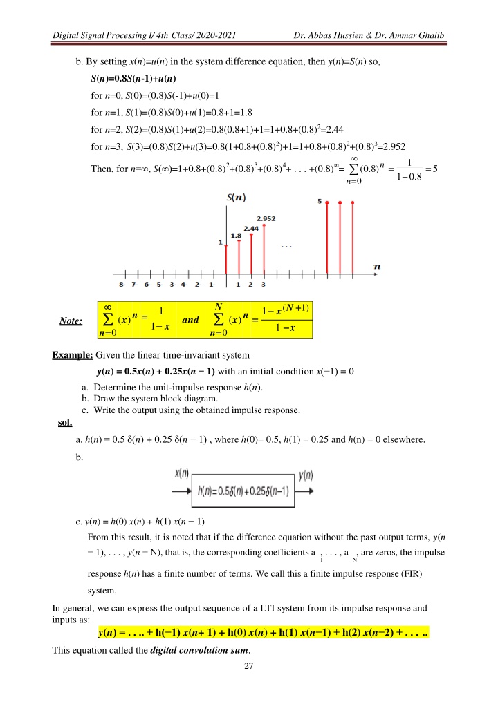
Digital Signal Processing I/ 4th Class/ 2020-2021 Dr. Abbas Hussien & Dr. Ammar Ghalib b. By setting x(n)=u(n) in the system difference equation, then y(n)=S(n) so, S(n)=0.8S(n-1)+u(n) for n=0, S(0)=(0.8)S(-1)+u(0)=1 for n=1, S(1)=(0.8)S(0)+u(1)=0.8+1=1.8 for n=2, S(2)=(0.8)S(1)+u(2)=0.8(0.8+1)+1=1+0.8+(0.8)2=2.44 for n=3, S(3)=(0.8)S(2)+u(3)=0.8(1+0.8+(0.8)2)+1=1+0.8+(0.8)2+(0.8)3=2.952 1 n n=0 2 3 4 = =5 Then, for n= , S( )=1+0.8+(0.8) +(0.8) +(0.8) + . . . +(0.8) = (0.8) 1 0.8 n= =0 N (x)n= =1 x(N + +1) 1 (x)n= = n= =0 and Note: 1 x 1 x Example: Given the linear time-invariant system y(n) = 0.5x(n) + 0.25x(n 1) with an initial condition x( 1) = 0 a. Determine the unit-impulse response h(n). b. Draw the system block diagram. c. Write the output using the obtained impulse response. sol. a. h(n) = 0.5 (n) + 0.25 (n 1) , where h(0)= 0.5, h(1) = 0.25 and h(n) = 0 elsewhere. b. c. y(n) = h(0) x(n) + h(1) x(n 1) From this result, it is noted that if the difference equation without the past output terms, y(n 1), . . . , y(n N), that is, the corresponding coefficients a , . . . , a , are zeros, the impulse 1 N response h(n) has a finite number of terms. We call this a finite impulse response (FIR) system. In general, we can express the output sequence of a LTI system from its impulse response and inputs as: y(n) = . . .. + h( 1) x(n+ 1) + h(0) x(n) + h(1) x(n 1) + h(2) x(n 2) + . . . .. This equation called the digital convolution sum. 27

Digital Signal Processing I/ 4th Class/ 2020-2021 Dr. Abbas Hussien & Dr. Ammar Ghalib Example: Given the difference equation y(n)= 0.25 y(n 1) + x(n) for n 0 and y( 1) = 0, a. Determine the unit-impulse response h(n). b.Draw the system block diagram. c. For a step input x(n) = u(n), find the output responses for the first three samples using the difference equation. sol. a. Let x(n) = (n), then h(n) = 0.25 h(n 1) + (n) To solve for h(n), we evaluate h(0) = 0.25 h( 1) + (0) = 0.25 ( 0 ) + 1 = 1 h(1) = 0.25 h(0) + (1) = 0.25 ( 1 ) + 0 = 0.25 h(2) = 0.25 h(1) + (2) = 0.25 ( 0.5 ) + 0 = 0.0625 With the calculated results, we can predict the impulse response as: n h(n) =( 0.25) u(n) = (n) + 0.25 (n 1) + 0.0625 (n 2) + . . . b. The system block diagram is given below c. From the difference equation and using the zero-initial condition, we have Notice that this impulse response h(n) contains an infinite number of terms in its duration due to the past output term y(n 1). Such a system as described in the preceding example is called an infinite impulse response (IIR) system. 28

Digital Signal Processing I/ 4th Class/ 2020-2021 Dr. Abbas Hussien & Dr. Ammar Ghalib Digital Convolution The Convolution Sum or Superposition Sum Representation of LTI Systems: The convolution allows us to find the output signal from any LTI processor in response to any input signal. We can find the output signal y(n) from an LTI processor by convolving its input signal x(n) with a second function representing the impulse response h(n) of the processor. The convolution sum or superposition sum of the sequences x(n) and h(n) can be represented by N= N +N -1. Where N = number of samples of x(n), N = number of samples of h(n), 1 2 1 and N= total number of samples. 2 This operation is represented symbolically as x(n)*h(n) Properties of Convolution: 1- Commutativity Convolution is a commutative operation, meaning signals can be convolved in any order. 2- Associativity (Cascaded Connection) Convolution is associative, meaning that convolution operations in series can be done in any order. 29

Digital Signal Processing I/ 4th Class/ 2020-2021 Dr. Abbas Hussien & Dr. Ammar Ghalib 3- Distributivity (Parallel Connection) Convolution is distributive over addition The digital convolution can be performed by graphical, table lookup, matrix by vector methods. Graphical Method: The convolution sum of two sequences can be found by using the following steps: Step 1. Obtain the reversed sequence h( - k). Step 2. Shift h( - k) by n samples to get h(n - k). If n 0, h( - k) will be shifted to the right by n samples; but if n < 0, h( - k) will be shifted to the left by n samples. Step 3. Perform the convolution sum that is the sum of the products of two sequences x(k) and h(n - k) to get y(n). Step 4. Repeat steps 1 to 3 for the next convolution value y(n). Example: Find the convolution of the two sequences x[n] and h[n] given by x[n] = {3, 1, 2} and h[n] = {3, 2, 1}. The bold number shows where n=0. Using: a. Direct method. b. Graphical method. sol. a. Using y[n] = = x[k]h[n k] k= = x[n] = {3, 1, 2} and h[n] = {3, 2, 1} Total number of samples N=N1+N2-1=3+3-1=5 samples. 30