Discrete Probability Distributions
A random variable is a numerical description of an outcome in an experiment, where it can be discrete or continuous. Examples and illustrations of discrete random variables with finite or infinite values are provided. Explore how probability distributions describe the likelihood of different outcomes and variables.

Download Presentation

Please find below an Image/Link to download the presentation.
The content on the website is provided AS IS for your information and personal use only. It may not be sold, licensed, or shared on other websites without obtaining consent from the author.If you encounter any issues during the download, it is possible that the publisher has removed the file from their server.
You are allowed to download the files provided on this website for personal or commercial use, subject to the condition that they are used lawfully. All files are the property of their respective owners.
The content on the website is provided AS IS for your information and personal use only. It may not be sold, licensed, or shared on other websites without obtaining consent from the author.
E N D
Presentation Transcript
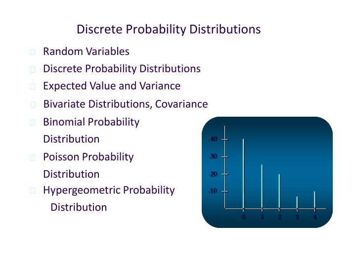
Discrete Probability Distributions Random Variables Discrete Probability Distributions Expected Value and Variance Bivariate Distributions,Covariance Binomial Probability Distribution PoissonProbability Distribution HypergeometricProbability Distribution .40 .30 .20 .10 0 1 2 3 4
RandomVariables A random variable is a numerical description of the outcome of an experiment. A discrete random variable may assume either a finite number of values or an infinite sequence of values. A continuous random variable may assume any numerical value in an interval or collection of intervals.
Discrete Random Variable with a Finite Number of Values Example: JSL Appliances Let x = number of TVs sold at the store in one day, where x can take on 5 values (0, 1, 2, 3,4) We can count the TVs sold, and there is a finite upper limit on the number that might be sold (which is the number of TVs in stock).
Discrete Random Variable with an Infinite Sequence of Values Example: JSL Appliances Let x = number of customers arriving in one day, where x can take on the values 0, 1, 2, . .. We can count the customers arriving, but there is no finite upper limit on the number that might arrive.
RandomVariables Type Question Random Variable x Family size x = Number of dependents reported on tax return Discrete x = Distance in miles from home to the store site Distance from home to store Continuous x = 1 if own no pet; = 2 if own dog(s) only; = 3 if own cat(s) only; = 4 if own dog(s) and cat(s) Own dog or cat Discrete
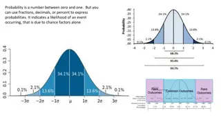
Discrete Probability Distributions The probability distribution for a random variable describes how probabilities are distributed over the values of the random variable. We can describe a discrete probability distribution with a table, graph, or formula.
Discrete Probability Distributions Two types of discrete probability distributions will be introduced. First type: experimental outcomes to determine probabilities for each value of the random variable. uses the rules of assigning probabilities to Second type: compute the probabilities for each value of the random variable. uses a special mathematicalformula to
Discrete Probability Distributions The probability distribution is defined by a probability function, denoted by f(x), that provides the probability for each value of the randomvariable. The required conditions for a discrete probability function are: f(x) > 0 f(x) = 1
Discrete Probability Distributions There are three methods for assign probabilities to random variables: the classical method, the subjective method, and the relative frequency method. The use of the relative frequency method to develop discrete probability distributions leads to what is called an empirical discrete distribution.
Discrete Probability Distributions Example: JSL Appliances Using past data on TV sales, a tabular representation of the probability distribution for TV sales was developed. Number of Days 80/200 x 0 1 2 3 4 f(x) .40 .25 .20 .05 .10 1.00 UnitsSold 0 1 2 3 4 80 50 40 10 20 200
Discrete Probability Distributions Example: JSL Appliances Graphical representation of probability distribution .50 .40 Probability .30 .20 .10 0 1 2 3 4 Values of Random Variable x (TVsales)
Discrete Probability Distributions In addition to tables and graphs, a formula that gives the probability function, f(x), for every value of x is often used to describe the probability distributions. Several discrete probability distributions specified by formulas are the discrete-uniform, binomial, Poisson, and hypergeometric distributions.
Discrete Uniform Probability Distribution The discrete uniform probability distribution is the simplest example of a discrete probability distribution given by a formula. The discrete uniform probability function is the values of the random are equallylikely f(x) =1/n variable where: n = the number of values the random variable may assume
Expected Value The expected value, or mean, of a random variable is a measure of its central location. E(x) = = xf(x) The expected value is a weighted average of the values the random variable may assume. weights are the probabilities. The The expected value does not have to be a value the random variable can assume.
Variance and Standard Deviation The variance summarizes the variability in the values of a random variable. Var(x) = 2 = (x - )2f(x) The variance is a weighted average of the squared deviations of a random variable from its mean. The weights are the probabilities. The standard deviation, , is defined as the positive square root of the variance.
Expected Value Example: JSLAppliances x 0 1 2 3 4 f(x) .40 .25 .20 .05 .10 xf(x) .00 .25 .40 .15 .40 1.20 E(x)= expected numberof TVs sold in aday
Variance Example: JSLAppliances x - (x - )2 (x - )2f(x) x f(x) -1.2 -0.2 0.8 1.8 2.8 Variance of daily sales = 2 =1.660 1.44 0.04 0.64 3.24 7.84 .40 .25 .20 .05 .10 0 1 2 3 4 .576 .010 .128 .162 .784 TVs squared Standard deviation of daily sales = 1.2884 TVs
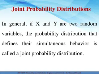
BivariateDistributions A probability distribution involving two random variables is called a bivariate probabilitydistribution. Each outcome of a bivariate experiment consistsof two values, one for each random variable. Example: rolling a pair of dice When dealing with bivariate probability distributions, we are often interested in the relationship between the random variables.
A Bivariate Discrete ProbabilityDistribution A company asked 200 of its employees how they rated their benefit package and job satisfaction. crosstabulation below shows the ratings data. The JobSatisfaction 1 (y) Benefits Package (x) 2 3 Total 1 2 3 28 22 2 26 42 10 4 58 34 32 98 44 Total 52 78 70 200
A Bivariate Discrete ProbabilityDistribution The bivariate empirical discrete probabilities for benefits rating and job satisfaction are shown below. JobSatisfaction 1 (y) Benefits Package (x) 2 3 Total .29 1 2 3 .14 .11 .13 .21 .02 .17 .49 .01 .05 .16 .22 1.00 Total .26 .39 .35
A Bivariate Discrete ProbabilityDistribution Expected Value and Variance for Benefits Package, x (x -E(x))2 (x - E(x))2f(x) f(x) xf(x) x -E(x) x 1 0.29 0.29 -0.93 0.8649 0.250821 2 0.49 0.98 0.07 0.0049 0.002401 3 0.22 0.66 1.07 1.1449 0.251878 E(x)= Var(x)= 1.93 0.505100
A Bivariate Discrete ProbabilityDistribution Expected Value and Variance for Job Satisfaction, y (y -E(y))2 (y - E(y))2f(y) f(y) yf(y) y -E(y) y 1 0.26 0.26 -1.09 1.1881 0.308906 2 0.39 0.78 -0.09 0.0081 0.003159 3 0.35 1.05 0.91 0.8281 0.289835 E(y)= Var(y)= 2.09 0.601900
A Bivariate Discrete ProbabilityDistribution Expected Value and Variance for Bivariate Distrib. (s -E(s))2 (s - E(s))2f(s) f(s) sf(s) s -E(s) s 2 0.14 0.28 -2.02 4.0804 0.571256 3 0.24 0.72 -1.02 1.0404 0.249696 4 0.24 0.96 -0.02 0.0004 0.000960 5 0.22 1.10 0.98 0.9604 0.211376 6 0.16 0.96 1.98 3.9204 0.627264 E(s)= Var(s)= 4.02 1.660552
A Bivariate Discrete ProbabilityDistribution Covariance for Random Variables x and y Varxy = [Var(x + y) Var(x) Var(y)]/2 Varxy= [1.660552 0.5051 0.6019]/2 =0.276776
A Bivariate Discrete ProbabilityDistribution Correlation Between Variables x and y = xy xy x y x 0.5051 0.710 y 0.6019 0.7758221 0.276776 0.526095 xy 0.526095 0.954 xy 0.7107038(0.7758221)
Binomial Probability Distribution Four Properties of a Binomial Experiment 1. The experiment consists of a sequence of n identical trials. 2. Two outcomes, success and failure, arepossible on each trial. 3. The probability of a success, denoted by p, does not change from trial to trial. stationarity assumption 4. The trials are independent.
Binomial Probability Distribution Our interest is in the number of successes occurring in the n trials. We let x denote the number of successes occurring in the n trials.
Binomial Probability Distribution Binomial Probability Function f(x)= n! px(1 p)(n x) x!(n x)! where: x = the number of successes p = the probability of a success on onetrial n = the number of trials f(x) = the probability of x successes in ntrials n! = n(n 1)(n 2) .. (2)(1)
Binomial Probability Distribution Binomial Probability Function n! f(x)= px(1 p)(n x) x!(n x)! Probability of a particular sequence of trialoutcomes with x successes in ntrials Number of experimental outcomes providingexactly x successes in ntrials
Binomial Probability Distribution Example: Evans Electronics is concerned about a low retention rate for its employees. management has seen a turnover of 10% of the employees annually. Evans Electronics In recentyears, Thus, for any employee chosen at random, management estimates a probability of 0.1 that the person will not be with the company next year. Choosing 3 employees at random, what is the probability that 1 of them will leave the company this year?
Binomial Probability Distribution Example: The probability of the first employee leaving and the second and third employees staying, denoted (S, F, F), is given by Evans Electronics p(1 p)(1 p) With a .10 probability of an employee leaving on any one trial, the probability of an employee leaving on the first trial and not on the second and third trials is given by (.10)(.90)(.90) = (.10)(.90)2 =.081
Binomial Probability Distribution Example: Two other experimental outcomes also result in one success and two failures. three experimental outcomes involving one success follow. Evans Electronics The probabilities for all Probability of Experimental Outcome Experimental Outcome p(1 p)(1 p) = (.1)(.9)(.9) =.081 (1 p)p(1 p) = (.9)(.1)(.9) =.081 (1 p)(1 p)p = (.9)(.9)(.1) =.081 (S, F,F) (F, S,F) (F, F,S) Total =.243
Binomial Probability Distribution Example: Evans Electronics Using the probability function Let: p = .10, n = 3, x =1 n! f ( x)=x!(n x)!px(1 p)(n x) f(1)= 3!(0.1)1 (0.9)2 = 3(.1)(.81)= 1!(3 1)! .243
Binomial Probability Distribution Using a tree diagram Example: Evans Electronics x 1stWorker 2ndWorker 3rdWorker L(.1) Prob. .0010 3 Leaves (.1) .0090 2 S(.9) Leaves (.1) L(.1) .0090 2 Stays(.9) 1 .0810 S(.9) L (.1) 2 .0090 Leaves (.1) Stays (.9) 1 .0810 S(.9) L(.1) 1 .0810 Stays(.9) 0 .7290 S(.9)
Binomial Probabilities and Cumulative Probabilities Statisticians have developed tables that give probabilities and cumulative probabilities for a binomial random variable. These tables can be found in statisticstextbooks. With modern calculators and the capability of statistical software packages, such tables are almost unnecessary.
Binomial Probability Distribution Using Tables of BinomialProbabilities p .05 .10 .15 .20 .25 .30 .35 .40 .45 .50 n x 3 0 1 2 3 .8574 .7290 .6141 .5120 .4219 .3430 .2746 .2160 .1664 .1250 .1354 .2430 .3251 .3840 .4219 .4410 .4436 .4320 .4084 .3750 .0071 .0270 .0574 .0960 .1406 .1890 .2389 .2880 .3341 .3750 .0001 .0010 .0034 .0080 .0156 .0270 .0429 .0640 .0911 .1250
Binomial Probability Distribution Expected Value E(x) = = np Variance Var(x) = 2 = np(1 p) StandardDeviation = np(1 p)
Binomial Probability Distribution Example: Expected Value Evans Electronics E(x) = np = 3(.1) = .3 employees out of 3 Variance Var(x) = np(1 p) = 3(.1)(.9) = .27 Standard Deviation = 3(.1)(.9) = .52 employees
Poisson Probability Distribution Poisson distribution occurs when there are events which do not occur as outcomes of a definite number of trials but occur at random points of time and space wherein our interest lies only in the number of occurrences of the event but not on non- occurrences. A Poisson distributed random variable is often useful in estimating the number of occurrences over a specified interval of time or space It is a discrete random variable that may assume an infinite sequence of values (x = 0, 1, 2, . . .).
Poisson Probability Distribution Examples of Poisson distributed random variables: the number of vehicles arriving at a toll booth in one hour Bell Labs used the Poisson distribution to model the arrival of phone calls.
Poisson Probability Distribution Poisson Probability Function xe f(x)= x! where: x = the number of occurrences in an interval f(x) = the probability of x occurrences in an interval = mean number of occurrences in an interval e = 2.71828 x! = x(x 1)(x 2) . . .(2)(1)
Poisson Probability Distribution Poisson Probability Function Since there is no stated upper limit for the number of occurrences, the probability function f(x) is applicable for values x = 0, 1, 2, without limit. In practical applications, x will eventually become large enough so that f(x) is approximately zero and the probability of any larger values of x becomes negligible.
Poisson Probability Distribution Example: Patients arrive at the emergency room of Mercy Hospital at the average rate of 6 per hour on weekend evenings. What is the probability of 4 arrivals in 30 minutes on a weekend evening? Mercy Hospital
Poisson Probability Distribution Using the probability function Example: MercyHospital = 6/hour = 3/half-hour, x =4 34(2.71828) 3 f (4)= = .1680 4 !
Poisson Probability Distribution Example: Mercy Hospital PoissonProbabilities 0.25 0.20 Probability Actually, thesequence continues: 11, 12, 13 0.15 0.10 0.05 0.00 1 2 3 4 5 6 7 8 9 10 0 Number of Arrivals in 30Minutes
Poisson Probability Distribution A property of the Poisson distribution is that the mean and variance are equal. = 2
Poisson Probability Distribution Example: Mercy Hospital Variance for Number of Arrivals During 30-Minute Periods = 2 =3
Hypergeometric Probability Distribution The hypergeometric distribution is closely related to the binomial distribution. When population is finite and sampling is done without replacement, so that the events are stochastically dependent, although random, we obtain hypergeometric distribution.
Hypergeometric Probability Distribution A box contains N marbles. Of these, r are drawn, marked and returned to the box. The contents of the Box are then thoroughly mixed. Next n marbles are drawn at random from the box, and the marked Marbles are counted. If x denotes the number of marked marbles, then what is the probability distribution of random variable x ?
Hypergeometric Probability Distribution For the hypergeometric distribution: the trials are not independent, and the probability of success changes fromtrial to trial.