Electrodynamics and Relativity Explained: Maxwell's Equations, Charged Particle Behavior, and More
Dive into the world of electromagnetism and relativity with a comprehensive guide covering topics such as Maxwell's Equations, charged particle dynamics, electrodynamic potentials, and practical applications like cyclotrons. Understand the fundamental principles and relationships in electromagnetic theory through illustrations and explanations provided in this insightful content.

Download Presentation

Please find below an Image/Link to download the presentation.
The content on the website is provided AS IS for your information and personal use only. It may not be sold, licensed, or shared on other websites without obtaining consent from the author. If you encounter any issues during the download, it is possible that the publisher has removed the file from their server.
You are allowed to download the files provided on this website for personal or commercial use, subject to the condition that they are used lawfully. All files are the property of their respective owners.
The content on the website is provided AS IS for your information and personal use only. It may not be sold, licensed, or shared on other websites without obtaining consent from the author.
E N D
Presentation Transcript
E&M and Relativity Eric Prebys, FNAL
Maxwells Equations In terms of total charge and current Q = = Gauss' Law enc E E d A S 0 0 = = 0 0 B B d A S B = = Faraday' Law s E E l d B d A t t C S E = + = + Ampere' Law s B J B l d I E d A 0 0 0 0 0 0 enclosed t t C S In terms of free charge an current = = ; D D S d A Q D E , f f enc D B H C D S = + l d = + ; H J I d A H , 0 f f enclosed t t Local effects of media USPAS, Knoxville, TN, January 20-31, 2013 Lecture 2 - Basic E&M and Relativity 2
Example: Field in a permeable dipole Cross section of dipole magnet Integration loop g B g 1 in gap l d = l d + H B 0 steel path steel C B g gap = I enclosed 0 msteel mgap N I 0 turns B gap g USPAS, Knoxville, TN, January 20-31, 2013 Lecture 2 - Basic E&M and Relativity 3
Electrodynamics and Electrodynamic Potentials We can write the electric and magnetic fields in terms of Vector and Scalar potentials B = ( ) , A r t A = E t Particle dynamics are governed by the Lorentz force law ( dt ) d p d v = + = = ; for F e E v B m v c dt d p = relativist ; ically correct dt USPAS, Knoxville, TN, January 20-31, 2013 Lecture 2 - Basic E&M and Relativity 4
Cyclotron (1930s) A charged particle in a uniform magnetic field will follow a circular path of radius side view top view B B mv = ( ) v c qB v 2 = f Cyclotron Frequency qB 2 = (constant! ) ! m f 2 qB = = s m Red box = remember! For a proton: = 15 2 . [ MHz ] fC B T Accelerating DEES USPAS, Knoxville, TN, January 20-31, 2013 5 Lecture 2 - Basic E&M and Relativity
Relativity Some Handy Relationships (homework) Basics v b =pc c E 1 dg = bg db b dp p 3db dp p dE E 2 1 =1 g2 =1 b2 = momentum p mv = 2 total energy E mc = 2 kinetic energy K E mc ( ) ( )2 2 = + 2 2 E mc pc A word about units For the most part, we will use SI units, except Energy: eV (keV, MeV, etc) [1 eV = 1.6x10⁻¹⁹ J] Mass: eV/c2 [proton = 1.67x10⁻²⁷ kg = 938 MeV/c2] Momentum: eV/c [proton @ =.9 = 1.94 GeV/c] USPAS, Knoxville, TN, January 20-31, 2013 Lecture 2 - Basic E&M and Relativity 6
4-Vectors and Lorentz Transformations We ll use the conventions ( , , , ct z y x P ) X E , , , p p p x y z c 1 0 0 0 0 1 0 0 = = A (velocity A along z axis) A 0 0 0 0 ( ) ct ( ) ( 2 2 2 = 2 2 2 X x y z c 2 ) E 2 2 = 2 x 2 y 2 z 2 P p p p mc c ( ) 2 2 = 2 P Meff c s Note that for a system of particles i We ll worry about field transformations later, as needed USPAS, Knoxville, TN, January 20-31, 2013 Lecture 2 - Basic E&M and Relativity 7
Some Handy Relationships Know all of these by heart because you re going to use them over and over! cos sin ) sin( B A B A = + + = + cos sin A B A B A B = sin( ) sin cos A cos sin A A B cos( ) cos cos sin sin A B B B = + cos( ) cos A cos A sin sin A B A B A B = sin 2 2 sin cos A = 2 cos 2 2 cos 1 A A 1 ( ) = + + sin cos sin( ) sin( ) A B A B A B 2 1 ( ) = + cos sin sin( ) sin( ) A B A B A B 2 1 ( ) = + + cos cos cos( ) cos( ) A B A B A B 2 1 ( ) = + sin sin cos( ) cos( ) A B A B A B 2 1 ( ) = + 2 cos 1 cos( 2 ) A A 2 1 ( ) ) A = 2 sin 1 cos( 2 A 2 USPAS, Knoxville, TN, January 20-31, 2013 Lecture 2 - Basic E&M and Relativity 8
Synchrotrons and beam rigidity The relativistic form of Newton s Laws for a particle in a magnetic field is: ( v q dt ) d p = = F B A particle in a uniform magnetic field will move in a circle of radius [ MeV/c B / ] 300 p p = [ m ] [ T ] qB In a synchrotron , the magnetic fields are varied as the beam accelerates such that at all points , and beam motion can be analyzed in a momentum independent way. It is usual to talk about he beam rigidity in T-m ( , ) ( ) B x t p t [ MeV/c ] p p Booster: (B )~30 Tm LHC : (B )~23000 Tm = ( ) ( )[ Tm ] B B 300 q USPAS, Knoxville, TN, January 20-31, 2013 9 Lecture 2 - Basic E&M and Relativity
Thin lens approximation and magnetic kick If the path length through a transverse magnetic field is short compared to the bend radius of the particle, then we can think of the particle receiving a transverse kick p p B l = = ( / ) qvBt qvB l v qBl and it will be bent through small angle p Bl = ( B ) p In this thin lens approximation , a dipole is the equivalent of a prism in classical optics. USPAS, Knoxville, TN, January 20-31, 2013 Lecture 2 - Basic E&M and Relativity 10
Field multipole expansion Formally, in a current free region Magnetic field is the gradient of a scalar = = 0 B B which satisfies Laplace s equation = = 2 0 0 B The general solution in two dimensions 2 2 ( ) = m m + = = + 0 ( , ) Re x y C x iy m 2 2 x y 0 USPAS, Knoxville, TN, January 20-31, 2013 Lecture 2 - Basic E&M and Relativity 11
Solving for B components ( ) = m 1 m = = + Re B mC x iy x m x 1 ( ) = m 1 m = = + Re B imC x iy y m y 1 Combining ( ) = n n + = + B iB K x iy y x n 0 USPAS, Knoxville, TN, January 20-31, 2013 Lecture 2 - Basic E&M and Relativity 12
Symmetry properties of mulitpoles ( ) = = n + = + = n in B iB K x iy K r e y x n n 0 0 n n = i = n in K e r e n n 0 n The phase angle m represents a rotation of each component about the axis. Set all m =0 for the moment = = = 0 0 ; dipole n B B K 0 x y = = = 1 ( ) 0 , r 0 ; ( ) 0 , r quadrupole n B r B r r K = 1 x y = ( , r ) 2 / = ; = ( B , ) 2 / r = 0 B r K B 1 x y + ( , ) ( , ) B , , x y x y = 2 2 ( ) 0 , r 0 ; ( ) 0 , r sextupole n B r B r r K 2 x y = = 2 ( , r ) 4 / ; = ( B , ) 4 / r 0 B r K B 2 x y + ( , ) 2 / ( , ) B , , x y x y USPAS, Knoxville, TN, January 20-31, 2013 Lecture 2 - Basic E&M and Relativity 13
Back to Cartesian Coordinates. Differentiate both sides n times wrt x x y iB B = + ( ) = n + K x iy n 0 n n B n B y + = ! x i n K n n n x x = = 0 x y = = 0 x y And we can rewrite this as = + n normal ( )( n 1 n ~ ) n + + ; B iB B B i x iy B B y x n n n y n ! x = 0 = = 0 x y n ~ B B n x n x skew = = 0 x y Normal terms always have Bx=0 on x axis. Skew terms always have By=0 on x axis. Generally define , 1 B B B B ~ B ~ B ~ B ~ B , , etc , 2 1 2 USPAS, Knoxville, TN, January 20-31, 2013 Lecture 2 - Basic E&M and Relativity 14
Expand first few terms ( ) B ~ B ~ B = + + + 2 2 ... B B B x y x y xy 0 y 2 ~ B ( ) ~ B ~ B = + + + + + 2 2 ... B x B y x y B xy 0 x 2 quadrupole sextupole dipole Note: in the absence of skew terms, on the x axis + + = B B 2 B 6 + + 2 3 n ... n ! B B B x x x x 0 y n sextupole quadrupole octupole dipole USPAS, Knoxville, TN, January 20-31, 2013 Lecture 2 - Basic E&M and Relativity 15
Application of Multipoles Dipoles: bend Quadrupoles: focus or defocus B B x y y x A positive particle coming out of the page off center in the horizontal plane will experience a restoring kick lx ( ) Bx x l B = ( ) ( ) B B ( ) B = f ' B l USPAS, Knoxville, TN, January 20-31, 2013 Lecture 2 - Basic E&M and Relativity 16
Sextupoles Octupoles In a similar way, octupoles have a field given by 1 ) ( B x By = Sextupole magnets have a field (on the principle axis) given by 1 = 2 3 ( ) By x B x x 2 6 So high amplitude particles will see a different average gradiant One common application of this is to provide an effective position- dependent gradient. B B y y x x x x max 2 max x = Beff x B = Beff B 2 17 Lecture 2 - Basic E&M and Relativity USPAS, Knoxville, TN, January 20-31, 2013


")