Forecasting Energy Market Series Using Econometric Models and Machine Learning Techniques
Modeling and forecasting hydrocarbon time series, particularly natural gas and crude oil, is crucial for various sectors impacted by hydrocarbons. The study compares econometric and machine learning techniques, explores volatility spillover between oil and stock returns, incorporates macroeconomic factors for accurate prediction, and emphasizes the benefits of accurate predictions for stakeholders.

Download Presentation

Please find below an Image/Link to download the presentation.
The content on the website is provided AS IS for your information and personal use only. It may not be sold, licensed, or shared on other websites without obtaining consent from the author.If you encounter any issues during the download, it is possible that the publisher has removed the file from their server.
You are allowed to download the files provided on this website for personal or commercial use, subject to the condition that they are used lawfully. All files are the property of their respective owners.
The content on the website is provided AS IS for your information and personal use only. It may not be sold, licensed, or shared on other websites without obtaining consent from the author.
E N D
Presentation Transcript
Forecasting Energy Market Series Using Econometric Models and Machine Learning Techniques SPYRIDON MASTRODIMITRIS GOUNAROPOULOS SUPERVISED BY: IOANNIS VRONTOS
PROBLEM STATEMENT AND IMPORTANCE OF STUDY Modeling and forecasting hydrocarbon time series more specifically natural gas and crude oil Hydrocarbons play an essential part in the modern economy by affecting directly and indirectly large sectors. Studying the advantages of econometric and alternative machine learning techniques comparisons Volatility spillover between oil and stock returns exists and is significant. Oil and Gas are significantly influenced by external effects making their accurate prediction a challenging while making Incorporating multiple macroeconomic factors including event indicators as predictive variables to improve prediction accuracy and show the impact of exogenous effects The ability to make accurate predictions greatly benefit hydrocarbon producing countries, corporations, the petrochemicals sector, provide a better protection from systemic risk to investors and support the consumer
LITERATURE REVIEW 1984 First Examples of Economic Series Predictions with ML 1993 2019 1997 Publicing of LSTMs by Hochreiter and Schmidhuber 2001 2017 2016 1982 Introduction of GARCH and by Engle and Bolleslev Introduction of GJRGARCH by Glosten, Jannathan and Runkle 1951 1991 Introduction of Temporal Fusion Transformers by Lim et al. Introduction of Random Forest by Breiman Introduction of Transformers by Vaswani et al. Introduction of XGBoost by Chen and Guestrin Introduction of ARMA by Whittle Introduction of EGARCH by Nelson
Data Our dependent variables were the Monthly and Quarterly prices for WTI, EUNG and ASIANG As external economic variables in a monthly frequency were selected the Equity Market Volatility Tracker, the Economic Policy Uncertainty Index for Europe and for the USA, the Current General Business Conditions for New York Index, the 3-Month Treasury Bill Secondary Market Rate, the Infectious Disease Tracker and the Global price of Nickel. On a quarterly frequency were selected the US Gross Domestic Product, the EU19 Gross Domestic Product, the Japanese Gross Domestic Product, the Equity Market Volatility Tracker, the Economic Policy uncertainty Index for Europe and for the USA, the 3-Month Treasury Bill Secondary Market Rate, the Infectious Disease Tracker All of our data were collected from the FRED datasets Conducted collinearity tests (e.g. variance inflation factor (VIF)) and kept variables uncorrelated with each other. After the variable selection the predictive variables were differentiated to achieve stationarity. To provide evidence that the new series were indeed stationary and could be used in our analysis. The tests were the Augmented Dickey Fuller (ADF) test and the Kwiatkowski Phillips Schmidt Shin (KPSS) test.
Oil and Gas The news always show a great impact e.g. the 2009 economic crisis, the American Oversupply of 2014, the Covid19 lockdowns in 2020, the Russian military exercises on the Ukrainian border in 2021, the start of the SMO and the destruction of Nord Stream in 2022
AUTOREGRESSIVE AND HETESKEDASTIC MODELS Linear Multiple Regression Autoregressive moving average model with: Generalized Autoregressive Heteroscedasticity (GARCH) with the ability to model time-varying volatility, modeling the changing future conditional variances based on past variances and past squared observations, can capturing periods of swings and calm in financial markets Integrated Generalized Autoregressive Heteroscedasticity (IGARCH) variant of the GARCH model. Unlike the standard GARCH model, which assumes that past shocks' impact on volatility decays over time. In the IGARCH model, the sum of the autoregressive and moving average coefficients is constrained to equal one, implying that shocks to the conditional variance have a permanent effect on future volatility Exponential Generalized Autoregressive Heteroscedasticity (EGARCH) assume that the main factor in determining future volatility is the magnitude and not the positivity or negativity of expected returns. Unlike GARCH, which could imply non-negative coefficients to ensure that the conditional variance is positive, the EGARCH model directly models the logarithm of the variance allowing for the accommodation of asymmetric effects of positive and negative shocks on volatility. GJR Generalized Autoregressive Heteroscedasticity (GJR GARCH) its key feature the introduction of an additional term in the variance equation to model the asymmetric response of volatility to positive and negative shocks.
MACHINE LEARNING MODELS Ensemble Learning Methods Random Forest, operates by producing multiple parallel decision trees that are then bootstrapped to a superior predictor. Its main advantage is its ability to capture complex nonlinear relationships and interactions between lagged variables without the need for explicit model specification as in traditional econometric models. XGBoost, also tree-based ensemble technique but instead of bagging it uses boosting and more specifically the GBM algorithm to gradually improve the new produced models based on the errors of wear models. It shares many of the advantages of the Random Forest combined with an improved performance for large datasets Deep Learning Methods Long Short-Term Memory, an improved RNN that solves the problem of vanishing gradient with the use of gates (forget, input, and output), LSTMs can remember or forget particular timesteps if deemed necessary, building the long-term dependency parameter matrix. Temporal Fusion Transformer, is a very complex attention-based architecture that combines high-performance multi-horizon forecasting with interpretable insights into temporal dynamics. The TFT utilizes recurrent layers, self-attention layers, and gating layers to learn temporal relationships at different scales and select relevant features for the forecasting task
PREDICTIVE VARIABLES Quarterly WTI EUNG ASIANG Regression X GARCH X IGARCH X RF X XGBOOST X LSTM X Regression X X X GARCH X X IGARCH X RF X X X XGBOOST X LSTM X X X Regression X GARCH X IGARCH X RF X XGBOOST X LSTM X LAG1 LAG2 LAG3 LAG4 USAGDP X X X X X X X X X X X X X Equity Market Volatility 3-Month Treasury Bill Infectious Disease Tracker COV19 RUWAR X X X X X X X X X X X X X X X X X X X X X X X X X X X Monthly WTI EUNG ASIANG RF X LSTM X RF X RF X Regression X GARCH X IGARCH X EGARCH X XGBOOST X Regression X GARCH X IGARCH X EGARCH X XGBOOST X LSTM X Regression X GARCH X IGARCH X EGARCH X XGBOOST X LSTM X LAG Equity Market Volatility Economic Policy Uncertainty Europe NY Business Conditions 3-Month Treasury Bill Infectious Disease Tracker Nickel COV19 RUWAR X X X X X X X X X X X X X X X X X X X X X X X X X X X X X
PREDICTIVE VARIABLES CONCLUSIONS Machine Learning models used more of our predictive variables The models for monthly data are less prone to incorporate other predictive variable Event Indicators were of higher importance for quarterly predictions Past quarters returns had greater predictive ability for the European market compared to the Asian or The American The Asian natural gas market less in common with the European than the American Crude The main predictive variables for the monthly data are the GDP of the USA and the Infectious Disease Tracker while the event variables were selected but only from the ML models The main predictive variables for the monthly data are Economic Policy Uncertainty and the Infectious Disease Tracker, for the European Market the event indicators show higher importance In general models with too many variables do not necessarily show better performance
MULTIPLE REGRESSION VIOLATION OF ASSUMPTIONS Independence of observations, apriori not true but also seen autocorrelation plot of the residuals from partial Homoscedasticity, violated as seen by the autocorrelation plot of the residuals Residual Normality, seen in the quantile quantile plot and proved by normality testing (Shapiro-Wilk)
REGRESSION WITH AUTOCORRELATED ERRORS AND CONDITIONAL HETEROSCEDASTICITY COMPONENTS
EFFECTS ON THE RESIDUALS We detect not autocorrelations or partial autocorrelations for the residuals. The lags that exceed the significance thresholds, we conducted Ljung-Box tests and significance as a result they are mere noise found no statistical The autocorrelation and partial autocorrelation graphs of the squared residuals show no heteroskedasticity By appling in our model a generalized error distribution we fixed the problem of Residual Normality, as seen in the quantile quantile plot and proven to be normal by a Shapiro-Wilk normality test.
CONCLUSIONS GARCH even after 40 years still offer reliable and accurate results to a complex problem Of all machine learning models the newest Temporal Fusin Transformers proves to have significant potential if not to replace old techniques to complement them Machine learning models in certain conditions can achieve comparable results to GARCH The carefool selection of macroeconomic predictive variables such as GDP growth, Policy Uncertainty Infectious Diseases Tracker can improve our predictions The incorporation of event indicators to our models can improve and update our models to current conditions The forecasting of a return that so much dependent on exogenous and unpredictable factors is a still to this day a difficult challenge
THANK YOU FOR YOUR TIME! What's past is prologue What's past is prologue William Shakespeare
LINEAR REGRESSION Based on the Least Squares method and incorporated into statistics by Francis Galton and Karl Pearson in the beginning of the 20th century is not the most modern nor complex method To provide accurate and robust results many assumptions exist: A linear relationship between the dependent and independent variables Independence of residuals, where residuals are the difference between observed and predicted values Normality of Residuals Homoscedasticity, meaning that the variance of errors is constant and does not fluctuate over time All of the above assumptions are violated to varying degrees in our energy series data making the linear regression incompatible to the nature of our problem and yet an important checkpoint for the rest of the models to surpass
AR MA An AR model predicts future behavior of a time series based on its past behavior, with the assumption that past values have a linear influence on future values Unlike the Autoregressive AR model, the MA model bases future values on past forecast errors, essentially capturing the shocks or noise in the time series Both require stationarity, meaning that the statistical properties of the series such as mean and variance remain constant over time. Also components such as seasonality have been detected and removed The ARMA model is the combination of the two components offering a more flexible and all encompassing solution ? ? ???? ? ??= ? + ???? ?+ ?=1 ?=1
GARCH The ARIMA model is unable to handle changing variance, this is why adding GARCH components is particularly useful when studying financial time series where the volatility changes over time The Generalized Autoregressive Conditional Heteroskedasticity by having the ability to model time-varying volatility, modeling the changing future conditional variances based on past variances and past squared observations, can capturing periods of swings and calm in financial markets Incorporating GARCH allows for more accurate forecasts by modeling not just the conditional mean (ARIMA) but also the conditional variance ? ? 2 2 ??2= ?0+ ???? ? + ???? ? ?=1 ?=1
IGARCH The Integrated Generalized Autoregressive Conditional Heteroskedasticity, is a variant of the GARCH model designed to address certain characteristics of financial time series data, particularly the long memory in volatility The main concept is that shocks to the volatility can have a persistent, undiminishing effect over time. Unlike GARCH where volatility tends to revert to a long-term mean, IGARCH implies that there is no mean reversion in volatility, reflecting the idea that financial markets can exhibit periods of sustained high or low volatility. This is particularly relevant for financial time series where significant events can have long-lasting effects The lack of mean reversion may unrealistic for all financial time series and the assumption of permanent shocks might lead to overestimation of future volatility, especially over longer horizons ? ? ??+ ??= 1 ?=1 ?=1
EGARCH The Exponential Generalized Autoregressive Conditional Heteroskedasticity model is another variant of the GARCH developed in order to capture certain characteristics, the particularly the asymmetries in and the possibility of heavy-tailed distributions Unlike the standard GARCH model, which models the conditional variance directly, the EGARCH model specifies the logarithm of the conditional variance. This approach ensures that the conditional variance is always positive, regardless of the parameter values, addressing a limitation of the basic GARCH model where the variance could become negative if the parameters took certain values The EGARCH model is complex than the GARCH, which can make parameter estimation and model interpretation more challenging, also can be sensitive to the initial values used in the estimation process and to the specification of the mean equation ? ? 2 log ??2= ?0+ ??? ?? ? + ??log ?? ? ?=1 ?=1
GJR-GARCH The GJR-GARCH model, named after its developers Glosten, Jagannathan, and Runkle, is an extension of GARCH. It was designed to account for the leverage effect, where negative returns tend to lead to higher subsequent volatility compared to positive returns of the same magnitude, a phenomenon commonly observed in financial markets This asymmetry in volatility response is not captured by the standard GARCH model, making the GJR-GARCH model particularly useful for certain financial time series On the other hand for time series with a less pronounced leverage effect GJR GARCH is possible to be less than an ideal fit ? ? ? 2 2 2 ??2= ?0+ ???? 1 + ???? ? + ???? ? ?? ? ?=1 ?=1 ?=1
RANDOM FOREST Random Forest is a versatile machine learning algorithm that can also be applied to time series data, although it is not inherently designed for this type of data. Random Forest is an ensemble learning method that operates by constructing a multitude of decision trees during training. The final prediction is made based on the average of these decision trees. A significant advantage of the Random Forest is that it can capture complex nonlinear relationships in the data, making it suitable for diverse datasets, including time series. Random Forests is less prone to overfitting due to its ensemble approach and can handle a large number of features and complex data relationships.
XGBOOST Xtreme Gradient Boosting, is a highly efficient and scalable implementation of gradient boosted trees designed for speed and performance Gradient boosting builds models in a stage-wise fashion as an ensemble of weak prediction models, typically decision trees Unlike traditional gradient boosting that grows trees greedily, XGBOOST uses a depth-first approach and prunes trees using the max depth parameter, enhancing flexibility and efficiency Gradient boosting inherently focuses on modeling the residuals of the data. At each iteration, a new model is trained to predict the residuals from the previous models, effectively refining the predictions step by step.
LSTM Long Short-Term Memory networks are a special kind of Recurrent Neural Network (RNN) capable of learning long-term dependencies. LSTMs have the ability to capture temporal dynamics and relationships over different time intervals The core of an LSTM unit is the memory cell which can maintain its state over time, making LSTMs capable of remembering and accessing information from the past. This is crucial for time series forecasting where past information is key to predicting future values LSTMs use three types of gates to control the flow of information input gates, output gates, and forget gates. These gates determine what information should be remembered or forgotten, thus enabling LSTMs to learn long-term dependencies and avoid issues like vanishing gradients Some disadvantages of the LSTM are the computational intensity at deep networks and large datasets, they require careful tuning and has overfitting problems on limited data
TEMPORAL FUSION TRANSFORMERS TFTs provide insights into the forecasting process by highlighting which features are most important for predictions and how these relationships evolve over time, addressing a common challenge in deep learning models related to interpretability Through the use of dual-stage attention mechanisms and variable selection networks, TFTs can dynamically focus on the most relevant input features and past time steps, enhancing model accuracy by adaptively learning from the most informative parts of the data TFTs are designed to accommodate various types of inputs, including static and dynamic (time-varying) features, as well as known future inputs, making them highly flexible and capable of handling complex, real-world time series forecasting tasks The sophisticated architecture and mechanisms of TFTs, while powerful, lead to increased computational complexity. This can result in higher demands for computational resources and longer training time along with careful tuning