Forecasting Unemployment Trends in the Free State Province

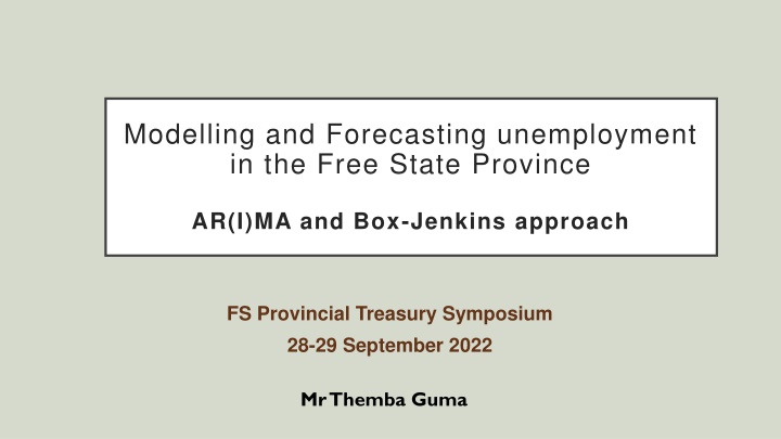
Modelling and Forecasting unemployment in the Free State Province AR(I)MA and Box-Jenkins approach FS Provincial Treasury Symposium 28-29 September 2022 Mr Themba Guma

Introduction & Objectives NDP sets unemployment rate at ambitious targets of 14% and 6% by 2020 and 2030. Whilst Sustainable Development Growth (SDG) seeks to achieve full employment economies by 2030. The main objectives of this study are threefold: o To determine the best or suitable AR(I)MA model for estimating Free State unemployment data time series o To forecast unemployment in the province of the Free State o To contribute to foundations of evidence based decision making, policy, and planning

Methodology (1) AR(I)MA Model AR, MA, or combined ARMA model are used for univariate time series modelling. Autoregressive Integrated Moving Average model (ARIMA) is applicable where there is a need for transformation of the time series. Autoregressive (AR): ??= ? + ?1?? 1+ ?2?? 2+ ......+ ???? ?+ ?? Moving Average (MA): ??= + ?+ ?1 ? 1+ ?2 ? 2+ ......+?? ? ? Combined (ARMA): ??= ? + ?1?? 1+ ?2?? 2+ ......+ ???? ?+ ?+ ?1 ? 1+ ?2 ? 2+ ......+?? ? ?

Methodology (2) Visual inspection Forms the base for insights Stationarity Stationarity - statistical properties of underlying generating stochastic process such as the mean, variance and autocorrelation / covariance that remain constant over time (t). OR when probability distribution function (pdf) remains unchanged over time. Dickey-Fuller (DF) Augmented Dickey- Phillips Perron (PP) Kwiatkowski Phillips Fuller (ADF) Schmidt Shin (KPSS) KPSS is a stationarity test DF, ADF and PP are also called non stationary or unit root tests Ho: variable a unit root ??: variable a unit root ??: variable a unit root ??: variable is stationary Non-stationarity Differencing method - ARIMA

Methodology (3) Box-Jenkins approach Identification Use of Correlogram Pattern of Auto Correlation Function (ACF) and Partial (PACF) For ARMA(1,1) Geometric decay after lag 1. Maybe oscillating for b <0) Estimation Significance of coefficients: model producing most significant coefficient (p-values<0.05) Tradeoff of fit vs parsimony Akaike Information Criterion (AIC) and Schwartz Bayesian Criterion (SBC) Approach- initial guesses about the model with a parsimonious low order AR Diagnostic checking Serial correlation- no autocorrelation or serial correlation / achieving white noise residuals Heteroscedasticity / Homoscedasticity inverse roots of AR/MA characteristic polynomial - lie inside the unit circle Structural break Dummy variable

Methodology (4) Forecasting Within the sample approach 2008Q1 to 2020Q2 Fan chart graph showing 30%, 60% and 90% confidence bands. Forecast evaluation for errors BIAS, MSE, SE, RMSE, MAE, MAPE Expanding window and Rolling window strategies 4 year horizon

Results (1) - Stationarity DFS_UNEMPLOYMENT_RATE Free State unemployment rate 5.0 45.0 2.5 40.0 35.0 0.0 30.0 -2.5 25.0 -5.0 20.0 Differenced 15.0 -7.5 10.0 -10.0 5.0 -12.5 0.0 2008Q1 2008Q3 2009Q1 2009Q3 2010Q1 2010Q3 2011Q1 2011Q3 2012Q1 2012Q3 2013Q1 2013Q3 2014Q1 2014Q3 2015Q1 2015Q3 2016Q1 2016Q3 2017Q1 2017Q3 2018Q1 2018Q3 2019Q1 2019Q3 2020Q1 2020Q3 2021Q1 2021Q3 2022Q1 -15.0 08 09 10 11 12 13 14 15 16 17 18 19 20 Kwiatkowski-Phillips-Schmidt-Shin (KPSS) test Null Hypothesis: FS_UNEMPLOYMENT_RATE is stationary Exogenous: Constant, Linear Trend Bandwidth: 4 (Newey-West automatic) using Bartlett kernel Augmented Dickey-Fuller (ADF) test Phillips-Perron (PP) test Null Hypothesis: FS_UNEMPLOYMENT_RATE has a unit root Exogenous: Constant, Linear Trend Null Hypothesis: FS_UNEMPLOYMENT_RATE has a unit root Exogenous: Constant, Linear Trend Adj. t-Stat LM-Stat. 0.209772 KPSS test statistic Asymptotic critical values*: Prob.* 0.1523 1% level 5% level 10% level 0.216000 0.146000 0.119000 t-Statistic Prob.* 0.1142 PP test statistic -2.965217 ADF test statistic -3.115559

Results (2) - Model identification The Model without Dum Dependent Variable: D(FS_UNEMPLOYMENT_RATE) Variable C AR(1) MA(1) Coefficient 0.187639 0.107807 -0.743955 0.189408 Std. Error 0.114221 0.281673 0.175497 -4.239143 Mean dependent var Akaike info criterion Durbin-Watson stat t-Statistic 1.642775 0.382740 Prob. 0.1074 0.7037 0.0001 -0.002083 4.730001 1.517546 R-squared S.E. of regression 2.498851 F-statistic 5.257491 The Model with Dum Dependent Variable: D(FS_UNEMPLOYMENT_RATE) Variable C DUM AR(1) MA(1) Coefficient 0.241273 -12.68530 0.574758 -0.999148 Std. Error 0.061049 0.989441 0.149762 0.085632 t-Statistic 3.952089 -12.82068 3.837819 -11.66789 Prob. 0.0003 0.0000 0.0004 0.0000 Chow Breakpoint Test: 2020Q2 Null Hypothesis: No breaks at specified breakpoints Equation Sample: 2008Q2 2022Q2 F-statistic 7.366008 Prob. F(3,51) 20.51862 Prob. Chi-Square(3) 0.0003 0.0001 - R-squared S.E. of regression F-statistic 0.609870 1.753168 22.92768 Mean dependent var Akaike info criterion Durbin-Watson stat 0.002083 4.040381 1.964787 Log likelihood ratio Wald Statistic 140.2527 Prob. Chi-Square(3) 0.0000

Results (3) -Diagnostics Autocorrelation check Fit & residual 5 4 0 2 -5 0 -10 -2 -15 -4 08 09 10 11 12 13 14 15 16 17 18 19 20 Residual Actual Fitted Inverse Roots of AR/MA Polynomial(s) 1.5 Stability condition 1.0 0.5 AR roots MA roots 0.0 Heteroscadicity / homoscedasticity -0.5 -1.0 -1.5 -1 0 1

Results (3) Automatic Model Selection & Model rep Akaike Information Criteria (top 20 models) Model Selection Criteria Table Dependent Variable: D(FS_UNEMPLOYMENT_RATE) Date: 09/15/22 Time: 19:15 Sample: 2008Q1 2020Q2 Included observations: 49 Model LogL (1,1)(0,0) -95.768569 4.113003 (0,2)(0,0) -96.596168 4.146782 (2,1)(0,0) -95.688000 4.150531 (1,2)(0,0) -95.690628 4.150638 (0,1)(0,0) -97.964575 4.161819 (0,3)(0,0) -96.028980 4.164448 (2,2)(0,0) -95.676898 4.190894 (1,3)(0,0) -95.688468 4.191366 (1,0)(0,0) -98.804312 4.196094 (0,4)(0,0) -95.979099 4.203229 (3,1)(0,0) -95.984745 4.203459 (0,0)(0,0) -100.251019 4.214327 (2,0)(0,0) -98.301138 4.216373 (3,0)(0,0) -97.437108 4.221923 (1,4)(0,0) -95.528517 4.225654 (2,3)(0,0) -95.676827 4.231707 (3,2)(0,0) -95.676854 4.231708 (4,0)(0,0) -96.777745 4.235826 (3,3)(0,0) -94.942991 4.242571 4.26 4.24 4.22 AIC* BIC HQ 4.20 4.306046 4.339825 4.382182 4.382289 4.316254 4.396100 4.461154 4.461626 4.350529 4.473489 4.473719 4.330153 4.409416 4.453574 4.534522 4.540576 4.540577 4.506086 4.590048 4.186243 4.220023 4.238419 4.238526 4.220412 4.252336 4.293430 4.293902 4.254687 4.305765 4.305995 4.258271 4.289613 4.309811 4.342838 4.348892 4.348893 4.338363 4.374403 4.18 4.16 4.14 4.12 4.10 (1,1)(0,0) (0,2)(0,0) (2,1)(0,0) (1,2)(0,0) (0,1)(0,0) (0,3)(0,0) (2,2)(0,0) (1,3)(0,0) (1,0)(0,0) (0,4)(0,0) (3,1)(0,0) (0,0)(0,0) (2,0)(0,0) (3,0)(0,0) (1,4)(0,0) (2,3)(0,0) (3,2)(0,0) (4,0)(0,0) (3,3)(0,0) (4,1)(0,0) Model Representation Estimation Equation: ========================= D(FS_UNEMPLOYMENT_RATE) = C(1) + C(2)*DUM + [AR(1)=C(3),MA(1)=C(4),BACKCAST=2008Q3,ESTSMPL="2008Q3 2020Q2"] Substituted Coefficients: ========================= D(FS_UNEMPLOYMENT_RATE) = 0.241272862767 - 12.6853035792*DUM + [AR(1)=0.574758218559,MA(1)=- 0.999148335538,BACKCAST=2008Q3,ESTSMPL="2008Q3 2020Q2"]

Results (3) Forecasting Prediction mean unemploy ment rate 30% 60% 90% Confide nce band Period Confidenc e band Confidenc e band 44 Low High Low High Low Hig 40 h 32,7 32,7 32,7 32,7 32,7 32,7 32,7 32,7 32,7 32,7 32,8 32,8 32,8 32,8 32,8 32,8 2022Q3 31,9 31,8 31,7 31,6 31,5 31,4 31,4 31,3 31,3 31,2 31,2 31,2 31,1 31,1 31,1 31,1 33,9 34,0 34,1 34,2 34,3 34,4 34,4 34,5 34,6 34,6 34,6 34,7 34,7 34,8 34,8 34,8 30,6 30,4 30,1 29,9 29,7 29,6 29,4 29,3 29,2 29,1 29,0 28,9 28,9 28,8 28,8 28,7 34,8 35,2 35,4 35,6 35,8 36,0 36,1 36,3 36,4 36,5 36,6 36,6 36,7 36,8 36,9 36,9 28,0 36,3 27,5 37,0 27,1 37,5 26,6 38,0 26,3 38,3 26,0 38,7 25,7 38,9 25,2 39,2 25,4 39,4 25,2 39,6 25,0 39,8 24,9 40,0 24,8 40,1 24,7 40,3 24,6 40,4 24,5 40,5 2022Q4 36 2023Q1 2023Q2 2023Q3 32 2023Q4 2024Q1 2024Q2 28 2024Q3 2024Q4 2025Q1 24 2025Q2 2025Q3 I II III IV I II III IV I II III IV I II III IV I II III IV I II 2025Q4 2021 2022 2023 2024 2025 2026 2026Q1 2026Q2

Results (3) Forecasting assessment Expanding strategy HORIZON Bias MSE RMSE SE MAE MAPE h=1 0.255 0.065 0.256 0.014 0.255 0.007 h=2 0.434 0.189 0.434 0.022 0.434 0.013 h=3 0.601 0.362 0.602 0.030 0.601 0.017 h=4 0.759 0.577 0.759 0.037 0.759 0.022 Model prediction vs Known reported values 45.0 40.0 35.0 30.0 25.0 % 20.0 15.0 10.0 Rolling strategy 5.0 0.0 2020 Q3 2020 Q4 37.0 2021 Q1 36.9 2021 Q2 36.8 2021 Q3 36.7 2021 Q4 36.6 2022 Q1 36.5 2022 Q2 36.4 HORIZON Bias MSE RMSE SE MAE MAPE h=1 0.077 0.016 0.126 0.100 0.116 0.003 h=2 0.118 0.037 0.192 0.152 0.176 0.005 h=3 0.139 0.049 0.221 0.173 0.199 0.006 h=4 0.149 0.055 0.235 0.182 0.210 0.006 Model Prediction 37.1 Known values (reported) 35.5 33.4 35.6 36.5 38.1 36.7 31.1 32.4

CONCLUDING REMARKS - END