Generating Learned NB Model with 2 Mapper-CPUs
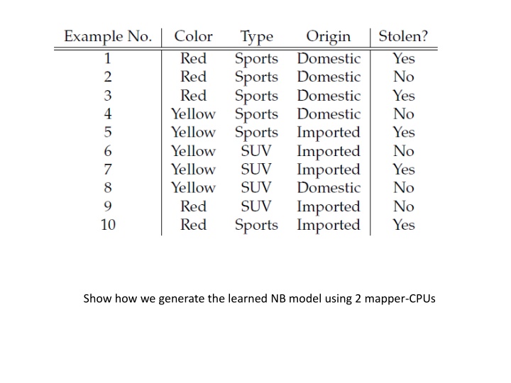
In this process, we utilize two mapper-CPUs to generate the learned Naive Bayes (NB) model. The mappers are configured to handle different aspects such as color, type, and origin of stolen items. The model is constructed based on the data collected on color, type, and origin, splitting into categories of 'yes' and 'no' to determine probabilities. The iterative process involves mapping, emitting successor nodes, calculating edge costs, and identifying maximum probabilities from predecessors. Adjustments are made iteratively until convergence, and finally, postprocessing involves the removal of adjacency lists to optimize the model.

Download Presentation

Please find below an Image/Link to download the presentation.
The content on the website is provided AS IS for your information and personal use only. It may not be sold, licensed, or shared on other websites without obtaining consent from the author.If you encounter any issues during the download, it is possible that the publisher has removed the file from their server.
You are allowed to download the files provided on this website for personal or commercial use, subject to the condition that they are used lawfully. All files are the property of their respective owners.
The content on the website is provided AS IS for your information and personal use only. It may not be sold, licensed, or shared on other websites without obtaining consent from the author.
E N D
Presentation Transcript
Show how we generate the learned NB model using 2 mapper-CPUs
Mapper-2 Mapper-1 Stolen? Colour | Stolen? Type | Stolen? Origin | Stolen?
Mapper-1 Class: yes=3, no=2, total=5 Colour Colour| yes: red=2, yellow=1, total=3 Colour| no: red=1, yellow=1, total=2 Type Type| yes: sports=3, SUV=0, total=3 Type| no: sports=2, SUV=0, total=2 Origin Origin| yes: domestic=2, imported=1, total=3 Origin| no: domestic=2, imported=0, total=2
C .8 A .75 uv .9 .5 H D .7 .8 B .9 .9 E A D H B C E A D H B C E
C 1 C 1 .8 .8 A 1 A .9 .75 .9 .75 .9 .5 .5 D 1 D 1 H H .7 B 1 .7 B .8 .8 .9 .8 .9 E 1 .9 E 1 .9 1. 2. C .72 C .72 .8 .8 A .9 A .9 .75 .9 .75 .9 .5 .5 D H D .56 H .64 .7 B .8 .7 .8 B .8 .9 .8 .9 E .9 E .9 3. .72 4. .72
init: For each node, node ID <1, -, {<succ-node-ID,edge-cost>}> map: take node ID < , next, {<succ-node-ID,edge-cost>}> For each succ-node-ID: emit succ-node ID {<node ID, * edge-cost>} emit node ID ,{<succ-node-ID,edge-cost>} reduce: := max prob. from a predecessor; next := that predec. emit node ID < , next, {<succ-node-ID,edge-cost>}> Repeat until no changes Postprocessing: Remove adjacency lists