Genomic Heritability Estimation Using Data" (53 characters)

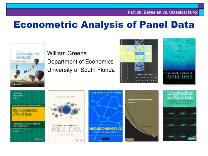
Part 26: Bayesian vs. Classical [1/45] Econometric Analysis of Panel Data William Greene Department of Economics University of South Florida

26. Modeling Heterogeneity in Classical Discrete Choice: Contrasts with Bayesian Estimation William Greene Department of Economics Stern School of Business New York University

Part 26: Bayesian vs. Classical [3/45] Abstract This study examines some aspects of mixed (random parameters) logit modeling. We present some familiar results in specification and classical estimation of the random parameters model. We then describe several extensions of the mixed logit model developed in recent papers. The relationship of the mixed logit model to Bayesian treatments of the simple multinomial logit model is noted, and comparisons and contrasts of the two methods are described. The techniques described here are applied to two data sets, a stated/revealed choice survey of commuters and one simulated data set on brand choice.

Part 26: Bayesian vs. Classical [4/45] Random Parameters Models of Discrete Choice Econometric Methodology for Discrete Choice Models Classical Estimation and Inference Bayesian Methodology Model Building Developments The Mixed Logit Model Extensions of the Standard Model Modeling Individual Heterogeneity Estimation of Individual Taste Parameters

Part 26: Bayesian vs. Classical [5/45] Useful References Classical Train, K., Discrete Choice Methods with Simulation, Cambridge, 2003. (Train) Hensher, D., Rose, J., Greene, W., Applied Choice Analysis, Cambridge, 2005. Hensher, D., Greene, misc. papers, 2003-2005, http://www.stern.nyu.edu/~wgreene Bayesian Allenby, G., Lenk, P., Modeling Household Purchase Behavior with Logistic Normal Regression, JASA, 1997. Allenby, G., Rossi, P., Marketing Models of Consumer Heterogeneity, Journal of Econometrics, 1999. (A&R) Yang, S., Allenby, G., A Model for Observation, Structural, and Household Heterogeneity in Panel Data, Marketing Letters, 2000.

Part 26: Bayesian vs. Classical [6/45] A Random Utility Model Random Utility Model for Discrete Choice Among J alternatives at time t by person i. Uitj j = Choice specific constant xitj = Attributes of choice presented to person (Information processing strategy. Not all attributes will be evaluated. E.g., lexicographic utility functions over certain attributes.) = Taste weights, Part worths, marginal utilities ijt = Unobserved random component of utility Mean=E[ ijt] = 0; Variance=Var[ ijt] = 2 = j + xitj + ijt

Part 26: Bayesian vs. Classical [7/45] The Multinomial Logit Model Independent type 1 extreme value (Gumbel): F( itj) = 1 Exp(-Exp( itj)) Independence across utility functions Identical variances, 2 = 2/6 Same taste parameters for all individuals exp( + 'x ) j itj Prob[choice j|i,t]= J (i) exp( + 'x ) t j itj j=1

Part 26: Bayesian vs. Classical [8/45] What s Wrong with this MNL Model? I.I.D. IIA (Independence from irrelevant alternatives) Peculiar behavioral assumption Leads to skewed, implausible empirical results Functional forms, e.g., nested logit, avoid IIA IIA will be a nonissue in what follows. Insufficiently heterogeneous: economists are often more interested in aggregate effects and regard heterogeneity as a statistical nuisance parameter problem which must be addressed but not emphasized. Econometricians frequently employ methods which do not allow for the estimation of individual level parameters. (A&R, 1999)

Part 26: Bayesian vs. Classical [9/45] Accommodating Heterogeneity Observed? Enter in the model in familiar (and unfamiliar) ways. Unobserved? The purpose of this study.

Part 26: Bayesian vs. Classical [10/45] Observable (Quantifiable) Heterogeneity in Utility Levels j U = + 'x + z + i jt j itj it ijt j exp( + 'x + z ) j itj it Prob[choice j|i,t]= J (i) exp( + 'x + z ) t j itj it j=1 Choice, e.g., among brands of cars xitj = attributes: price, features Zit = observable characteristics: age, sex, income

Part 26: Bayesian vs. Classical [11/45] Observable Heterogeneity in Preference Weights U = + x + z + + h + = h i j jt i j itj it ijt = i i k i, k k i exp( + x + z ) exp( + x + z ) i j j itj it Prob[choice j|i,t]= J (i) j=1 i t j itj it

Part 26: Bayesian vs. Classical [12/45] Quantifiable Heterogeneity in Scaling U = + 'x + z + j i jt j itj it ijt Var[ ]= exp( w ), = /6 2 j 2 1 2 j ijt it w wit it = observable characteristics: age, sex, income, etc. = observable characteristics: age, sex, income, etc.

Part 26: Bayesian vs. Classical [13/45] Heterogeneity in Choice Strategy Consumers avoid complexity Lexicographic preferences eliminate certain choices choice set may be endogenously determined Simplification strategies may eliminate certain attributes Information processing strategy is a source of heterogeneity in the model.

Part 26: Bayesian vs. Classical [14/45] Modeling Attribute Choice Conventional: Uijt = xijt. For ignored attributes, set xk,ijt =0. Eliminates xk,ijt from utility function Price = 0 is not a reasonable datum. Distorts choice probabilities Appropriate: Formally set k = 0 Requires a person specific model Accommodate as part of model estimation (Work in progress) Stochastic determination of attribution choices

Part 26: Bayesian vs. Classical [15/45] Choice Strategy Heterogeneity Methodologically, a rather minor point construct appropriate likelihood given known information M logL = = logL ( | data,m) i m 1 i M Not a latent class model. Classes are not latent. Not the variable selection issue (the worst form of stepwise modeling) Familiar strategy gives the wrong answer.

Part 26: Bayesian vs. Classical [16/45] Application of Information Strategy Stated/Revealed preference study, Sydney car commuters. 500+ surveyed, about 10 choice situations for each. Existing route vs. 3 proposed alternatives. Attribute design Original: respondents presented with 3, 4, 5, or 6 attributes Attributes four level design. Free flow time Slowed down time Stop/start time Trip time variability Toll cost Running cost Final: respondents use only some attributes and indicate when surveyed which ones they ignored

Part 26: Bayesian vs. Classical [17/45] Estimation Results

Part 26: Bayesian vs. Classical [18/45] Structural Heterogeneity Marketing literature Latent class structures Yang/Allenby - latent class random parameters models Kamkura et al latent class nested logit models with fixed parameters

Part 26: Bayesian vs. Classical [19/45] Latent Classes and Random Parameters Heterogeneity with res pect to 'latent' consumer classe s Q Pr(Choice ) = Pr(choice | class = q)Pr(class = q) i i q=1 i,choice exp(x exp(x ) class Pr(choice | class = q) = i,j xp(z ) exp(z ) i ) j=choice class i e q Pr(clas s = q|i) =F , e.g., F = i i,q i,q q=classes q Simple discrete random parameter variati on i,choice exp(x ) exp(x ) i Pr(choice | ) = i,j i i j=choice i i exp(z ) exp(z ) q Pr( = ) =F = ,q =1,...,Q i i q i,q q=classes q Q Pr(Cho ice ) = Pr(c hoice | = )Pr( ) i i q q q=1

Part 26: Bayesian vs. Classical [20/45] Latent Class Probabilities Ambiguous at face value Classical Bayesian model? Equivalent to random parameters models with discrete parameter variation Using nested logits, etc. does not change this Precisely analogous to continuous random parameter models Not always equivalent zero inflation models

Part 26: Bayesian vs. Classical [21/45] Unobserved Preference Heterogeneity What is it? How does it enter the model? U = + 'x + z + +w j ijt j itj it ijt i Random Parameters? Random Effects ?

Part 26: Bayesian vs. Classical [22/45] Random Parameters? Stochastic Frontier Models with Random Coefficients. M. Tsionas, Journal of Applied Econometrics, 17, 2, 2002. Bayesian analysis of a production model What do we (does he) mean by random?

Part 26: Bayesian vs. Classical [23/45] What Do We Mean by Random Parameters? Bayesian Classical Parameter Uncertainty? (A&R) Whose? Distribution defined by a prior? Whose prior? Is it unique? Is one right? Definitely NOT heterogeneity. That is handled by individual specific random parameters in a hierarchical model. Distribution across individuals Model of heterogeneity across individuals Characterization of the population Superpopulation? (A&R)

Part 26: Bayesian vs. Classical [24/45] Continuous Random Variation in Preference Weights U = = + x + z + + h +w + h +w Most treatments set = = +w i j ijt j itj it ijt i i i = k i,k k i i,k 0 i i exp( + x + z ) exp( + x + z ) i j j itj it Prob[choice j|i,t]= J (i) j=1 i t j itj it H eterogeneity arises from continuous variation in across individuals. (Classical and Bayesian) i

Part 26: Bayesian vs. Classical [25/45] What Do We Estimate? Classical f( i| ,Zi)=population Estimate , then E[ i| ,Zi)=cond l mean V[ i| ,Zi)=cond l var. Bayesian f( | 0)=prior L(data| )=Likelihood f( |data, 0)=Posterior E( |data, 0)=Posterior Mean V( |data, 0)=Posterior Var. Estimation Paradigm Exact More accurate ( Not general beyond this prior and this sample ) Estimation Paradigm Asymptotic (normal) Approximate Imaginary samples

Part 26: Bayesian vs. Classical [26/45] How Do We Estimate It? Objective Bayesian: Posterior means Classical: Conditional Means Mechanics: Simulation based estimator Bayesian: Random sampling from the posterior distribution. Estimate the mean of a distribution. Always easy. Classical: Maximum simulated likelihood. Find the maximum of a function. Sometimes very difficult. These will look suspiciously similar.

Part 26: Bayesian vs. Classical [27/45] A Practical Model Selection Strategy What self contained device is available to suggest that the analyst is fitting the wrong model to the data? Classical: The iterations fail to converge. The optimization otherwise breaks down. The model doesn t work. Bayesian? E.g., Yang/Allenby Structural/Preference Heterogeneity has both discrete and continuous variation in the same model. Is this identified? How would you know? The MCMC approach is too easy. It always works.

Part 26: Bayesian vs. Classical [28/45] Bayesian Estimation Platform: The Posterior (to the data) Density 0 Prior : f( | ) Likelihood : L( |data) f(data| ) Joint density: f( ,data| ) = L( |data)f( | ) 0 0 0 f( ,data| ) f(data) | ) 0 Posterior : f( |data, )= 0 L( |data)f( L( |data)f( | )d = 0 0 Posterior density of given data and prior

Part 26: Bayesian vs. Classical [29/45] The Estimator is the Posterior Mean E[ |data, ]= f( |data, ) d 0 0 L( |data)f( | ) L( |data)f( | )d 0 = d 0 Simulation based (MCMC) estimation: Empirically, 1 R R r=1 E[ ]= | known posterior population r This is not exact. It is the mean of a random sample.

Part 26: Bayesian vs. Classical [30/45] Classical Estimation Platform: The Likelihood Marginal: f( |data, ) Population Mean=E[ |data, ] i i = f( | )d i i i i = = a subvector of = Argmax L( ,i=1,...,N|data, ) i Estimator = Expected value over all possible realizations of i (according to the estimated asymptotic distribution). I.e., over all possible samples.

Part 26: Bayesian vs. Classical [31/45] Maximum Simulated Likelihood True log likelihood T t=1 L ( |data )= f(data | ) i i i i i i T t=1 L ( |data )= f(data | )f( | )d i i i i i i i i N i=1 logL= log L ( |data )f( | )d i i i i i i Simulated log likelihood 1 R N i=1 R r=1 logL = log L ( |data , ) S i iR i =argmax(logL ) S

Part 26: Bayesian vs. Classical [32/45] Individual Parameters ~ N( , ), i.e., = + w ~ N( , ), i.e., = + w ~ Inverse Wishart(G ,g ) i i i 0 0 0 0 0 0 =Posterior Mean =E[ | data, , ,G ,g ] Computed using a Gibbs sample (MCMC) i i 0 0 0 0

Part 26: Bayesian vs. Classical [33/45] Estimating i i In contrast, classical approaches to modeling heterogeneity yield only aggregate summaries of heterogeneity and do not provide actionable information about specific groups. The classical approach is therefore of limited value to marketers. (A&R p. 72)

Part 26: Bayesian vs. Classical [34/45] A Bayesian View: Not All Possible Samples, Just This Sample Based on any 'classical' random parameters model, E[ |This sample]= f( |data , )d i i i i i i = conditional mean in f( |data , ) = conditional mean conditioned on the data observed for individual i. i i = i L( |data )f( L( |data )f( | )d | ) d i i i i i i i i i i Looks like the posterior mean

Part 26: Bayesian vs. Classical [35/45] THE Random Parameters Logit Model Random U U = tility : + x + z + i i,j ijt i,j itj it ijt Random parameters: = + w + u = + w + u , a diagonal matrix Extensions: Correl ation: = Autocorrelation: u Str uctural pa rameters: =[ , , k i,k k i k i,k i i i triangular matrix = u +v eterogeneity : , a lower i,k,t i,k,t-1 i,k,t Variance H = , ] exp( f ) k i i,k k

Part 26: Bayesian vs. Classical [36/45] Conditional Estimators 1 R T t=1 N i=1 R r=1 =argmax log P ( | ,data ) i ijt ir it T t=1 L = P ( | ,data ) i i ijt i it (1/R) (1/R) P ( | ,data ) P ( | ,data ) t=1 ijt i T t=1 ijt i R r=1 R r=1 T t=1 ijt T t=1 ijt 1 R R r=1 i,k,r i it E[ |data ]= = w i,k i i,r i,k,r i it (1/R) (1/R) P ( | ,data ) P ( | ,data ) R r=1 R r=1 2 i,k,r T 1 R R r=1 it E[ | data ]= = w 2 i,k 2 i,k,r i i,r it 2 Var[ |data ]=E[ |data ]- E[ |data ] 2 i,k i,k i i i,k i E[ reasonable distribution |data ] 2 Var[ |data ] will encompass 95% of any i,k i i,k i

Part 26: Bayesian vs. Classical [37/45] Simulation Based Estimation Bayesian: Limited to convenient priors (normal, inverse gamma and Wishart) that produce mathematically tractable posteriors. Largely simple RPM s without heterogeneity. Classical: Use any distributions for any parts of the heterogeneity that can be simulated. Rich layered model specifications. Comparable to Bayesian (Normal) Constrain parameters to be positive. (Triangular, Lognormal) Limit ranges of parameters. (Uniform, Triangular) Produce particular shapes of distributions such as small tails. (Beta, Weibull, Johnson SB) Heteroscedasticity and scaling heterogeneity Nesting and multilayered correlation structures

Part 26: Bayesian vs. Classical [38/45] Computational Difficulty? Outside of normal linear models with normal random coefficient distributions, performing the integral can be computationally challenging. (A&R, p. 62) (No longer even remotely true) (1) MSL with dozens of parameters is simple (2) Multivariate normal (multinomial probit) is no longer the benchmark alternative. (See McFadden and Train) (3) Intelligent methods of integration (Halton sequences) speed up integration by factors of as much as 10. (These could be used by Bayesians.)

Part 26: Bayesian vs. Classical [39/45] Individual Estimates Bayesian exact what do we mean by the exact posterior Classical asymptotic These will be very similar. Counterpoint is not a crippled LCM or MNP. Same model, similar values. Atheorem of Bernstein-von Mises: Bayesian ------ > Classical as N (The likelihood function dominates; posterior mean mode of the likelihood; the more so as we are able to specify flat priors.)

Part 26: Bayesian vs. Classical [40/45] Extending the RP Model to WTP Use the model to estimate conditional distributions for any function of parameters Willingness to pay = i,time / i,cost Use same method R r R r T t T t (1/ ) (1/ ) ( ( | | , , ) ) R R WTP P P data data 1 R R = = 1 1 ir ijt ir it = = [ | ] E WTP data w WTP , i i i r ir = 1 r = = 1 1 ijt ir it

Part 26: Bayesian vs. Classical [41/45] What is the Individual Estimate? Point estimate of mean, variance and range of random variable i | datai. Value is NOT an estimate of i ; it is an estimate of E[ i| datai] What would be the best estimate of the actual realization i|datai? An interval estimate would account for the sampling variation in the estimator of that enters the computation. Bayesian counterpart to the preceding? Posterior mean and variance? Same kind of plot could be done.

Part 26: Bayesian vs. Classical [42/45] Methodological Differences Focal point of the discussion in the literature is the simplest possible MNL with random coefficients, exp( + x ) exp( + x ) i i,j itj P P rob[choice j|i,t]= J (i) j=1 i t i,j itj w w i,j i, j j = + i i This is far from adequate to capture the forms of heterogeneity discussed here. Many of the models discussed here are inconvenient or impossible with received Bayesian methods.

Part 26: Bayesian vs. Classical [43/45] A Preconclusion The advantage of hierarchical Bayes models of heterogeneity is that they yield disaggregate estimates of model parameters. These estimates are of particular interest to marketers pursuing product differentiation strategies in which products are designed and offered to specific groups of individuals with specific needs. In contrast, classical approaches to modeling heterogeneity yield only aggregate summaries of heterogeneity and do not provide actionable information about specific groups. The classical approach is therefore of limited value to marketers. (A&R p. 72)

Part 26: Bayesian vs. Classical [44/45] Disaggregated Parameters The description of classical methods as only producing aggregate results is obviously untrue. As regards targeting specific groups both of these sets of methods produce estimates for the specific data in hand. Unless we want to trot out the specific individuals in this sample to do the analysis and marketing, any extension is problematic. This should be understood in both paradigms. NEITHER METHOD PRODUCES ESTIMATES OF INDIVIDUAL PARAMETERS, CLAIMS TO THE CONTRARY NOTWITHSTANDING. BOTH PRODUCE ESTIMATES OF THE MEAN OF THE CONDITIONAL (POSTERIOR) DISTRIBUTION OF POSSIBLE PARAMETER DRAWS CONDITIONED ON THE PRECISE SPECIFIC DATA FOR INDIVIDUAL I.

Part 26: Bayesian vs. Classical [45/45] Conclusions When estimates of the same model are compared, they rarely differ by enough to matter. See Train, Chapter 12 for a nice illustration Classical methods shown here provide rich model specifications and do admit individual estimates. Have yet to be emulated by Bayesian methods Just two different algorithms. The philosophical differences in interpretation is a red herring. Appears that each has some advantages and disadvantages