Homogeneous and Non-homogeneous Linear Systems of Equations
Explore the concepts of homogeneous and non-homogeneous linear systems of equations, equilibrium solutions, and stability analysis through linear approximations. Dive into the graphical representations and critical point stability determinations in calculus and differential equations.

Download Presentation

Please find below an Image/Link to download the presentation.
The content on the website is provided AS IS for your information and personal use only. It may not be sold, licensed, or shared on other websites without obtaining consent from the author. If you encounter any issues during the download, it is possible that the publisher has removed the file from their server.
You are allowed to download the files provided on this website for personal or commercial use, subject to the condition that they are used lawfully. All files are the property of their respective owners.
The content on the website is provided AS IS for your information and personal use only. It may not be sold, licensed, or shared on other websites without obtaining consent from the author.
E N D
Presentation Transcript
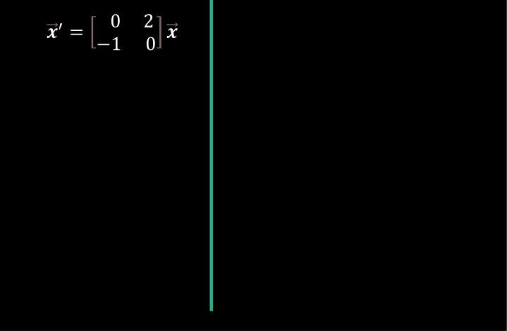
?= 0 2 0? 1
?= 0 2 0? 1 https://www.geogebra.org/m/abg8NJzF
Chapter 7: Homogeneous linear system of equations: x = Ax Section 9.2: Non-homogeneous linear system of equations: x = Ax + b To find equilibrium solutions, set x = 0: Suppose Aw + b = 0 for some constant vector w. Then x = w is a solution to x = Ax + b : [w] = 0 = Aw + b Thus x = w is an equilibrium solution. To determine its type, translate to the origin (or graph): Let u = x w. Then x = u + w (u + w) = A(u + w) + b u + w = Au + Aw + b u = Au
?= 0 2 0? ? = 0 2 0? + 4 3 1 1 https://www.geogebra.org/m/abg8NJzF
?= 0 2 0? ? = 0 2 0? + 4 3 1 1 https://www.geogebra.org/m/abg8NJzF
?= 0 2 0? ? = 0 2 0? + 4 3 1 1 https://www.geogebra.org/m/abg8NJzF
https://www.geogebra.org/m/abg8NJzF https://www.wolframalpha.com/input/?i=streamplot+%7B+x+-+xy%2C++-y+%2B+xy%7D
9.2 Calculus 1: Linear approx. = tangent line
Locally can be approximated by a stable center Locally can be approximated by an unstable saddle Nonlinear system of differential equations can be locally approximated by linear homog DE x = Ax
We will determine stability of these critical points in 9.3 via linear approximations. Can also determine graphically (but be careful): 2 equilibrium solutions Saddle Center (or slowly expanding or contracting spiral)
https://www.wolframalpha.com/ streamplot[{y, x^2}-1] streamplot[{y, x^2-1}, {x, -2, 2}, {y, -2, 2}] https://www.geogebra.org/m/abg8NJzF Streamplot shows small trajectories, while Slope fields direction fields show small portions of tangent lines.
? ? q 2= < 0 2= > 0 Complex roots 2 positive eigenvalues 2 negative eigenvalues Two real roots p Repeated roots q < 0 implies 1 positive and 1 negative eigenvalue Two complex roots Unstable
Center is stable, but not asymptotically stable Asymptotically stable Just need one positive expo- nential for Unstable