Introduction to Convolution and Image Processing

Concepts of convolution in image processing, Fourier spectrum, spatial filtering operations, noise cleaning techniques, edge detection, and the convolution theorem. Learn about various applications and properties of convolution, along with practical examples. Dive into the world of signal processing and enhance your understanding of filtering and image manipulation.

Download Presentation

Please find below an Image/Link to download the presentation.
The content on the website is provided AS IS for your information and personal use only. It may not be sold, licensed, or shared on other websites without obtaining consent from the author.If you encounter any issues during the download, it is possible that the publisher has removed the file from their server.
You are allowed to download the files provided on this website for personal or commercial use, subject to the condition that they are used lawfully. All files are the property of their respective owners.
The content on the website is provided AS IS for your information and personal use only. It may not be sold, licensed, or shared on other websites without obtaining consent from the author.
E N D
Presentation Transcript
To register to the mailing list: http://www.wisdom.weizmann.ac.il/~vision/courses/ 2017_1/intro_to_vision/index.html (or just google Weizmann Vision ).
Fourier Spectrum 2D Image
Convolution (continuou 1D discrete) s, : = * ( ) ( ) ( ) f g Good for: - Pattern matching - Filtering - Understanding Fourier properties x f g x d = 1 N = = ( ) ( ) f g x 0 (continuou 2D discrete) s, : = * ( , ) ( , ) ( , ) f g x y f g x y d d = = 1 1 N N = = 0 ( , ) ( , ) f g x y = 0
Convolution Properties Commutative: f*g = g*f Associative: (f*g)*h = f*(g*h) Homogeneous: f*( g)= f*g Additive (Distributive): f*(g+h)= f*g+f*h Shift-Invariant f*g(x-x0,y-yo)= (f*g) (x-x0,y-yo)
Spatial Filtering Operations Example 1 1 1 1 ( , ) 1 1 1 f x y 9 1 1 1 3 x 3 h(x,y) = 1/9 f(n,m) (n,m) in the 3x3 neighborhood of (x,y)
Noise Cleaning Salt & Pepper Noise 3 X 3 Average 5 X 5 Average 7 X 7 Average Median
Noise Cleaning Salt & Pepper Noise 3 X 3 Average 5 X 5 Average 7 X 7 Average Median
A very simplistic Edge Detector 1 ) ( ( , + ) 1 f x y 1 = ) 1 + ( , ( , ) f x y f x y ( , ) f x y = ( , 1 , ) f x y f x y 1 f Gradient magnitude f = f x derivative y derivative 2 2 x y + f f x y
The Convolution Theorem ( ) x ( ) x ( ) x ( ) x = f g f g and similarly: ( ) ( ) g x ( ) x ( ) x = f x f g Proof: Homework
Going back to the Noise Cleaning example 1 1 1 1 = 1 1 1 9 1 1 1 3 X 3 Average Salt & Pepper Noise Convolution with a rect Multiplication with a sinc in the Fourier domain =LPF (Low-Pass Filter) 7 X 7 Average 5 X 5 Average Wider rect Narrower sinc= Stronger LPF
Examples 2 = ( ) sinc f x What is the Fourier Transform of ? = ( ) (x f 2) = = { ( )} {sinc sinc} f x = rect {sinc} * {sinc} = * rect = * =
Image Domain Frequency Domain
The Sampling Theorem (developed on the board) Nyquist frequency, Aliasing, etc
Multi-Scale Image Representation Gaussian pyramids Laplacian Pyramids Wavelet Pyramids Good for: - pattern matching - motion analysis - image compression - other applications
Image Pyramid Low resolution High resolution
FastPattern Matching search search search search
The Gaussian Pyramid = ( * ) 2 G G gaussian Low resolution 4 3 gaussian blur = ( * ) 2 G G 3 2 blur = ( * ) 2 G G gaussian 2 1 blur = ( * ) 2 G G G gaussian 1 1 0 = Image G blur 0 High resolution
The Laplacian Pyramid expand( = i i G L expand( + = i i L G ) ) G G + 1 i Laplacian Pyramid L = Gaussian Pyramid + 1 i G G n n n G - 2 L = 2 G 1 L 1 - = G 0 L 0 - =
Laplacian ~ Difference of Gaussians - = DOG = Difference of Gaussians More details on Gaussian and Laplacian pyramids can be found in the paper by Burt and Adelson (link will appear on the website).
Computerized Tomography (CT) ( ) 2x p ( ) 1x p v F(u,v) u f(x,y) = ( ) ( ) 0 , u P u F (x ) p = ( ) ( , ) p x f x y dy
Computerized Tomography Original (simulated) 2D image 8 projections- Frequency Domain 120 projections- Frequency Domain Reconstruction from 120 projections Reconstruction from 8 projections
End of Lesson... Exercise#1 -- will be posted on the website. (Theoretical exercise: To be done and submitted individually) To register to the mailing list: http://www.wisdom.weizmann.ac.il/~vision/courses/ 2017_1/intro_to_vision/index.html (or just google Weizmann Vision ).


")