Introduction to Hidden Markov Models

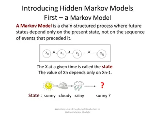
Hidden Markov Models (HMM) are a key concept in the field of Natural Language Processing (NLP), particularly in modeling sequences of random variables that are not independent, such as weather reports or stock market numbers. This technology involves understanding properties like limited horizon, time invariance, and transition matrices, making it a valuable tool for various applications. With examples, explanations of visible and hidden Markov models, and their uses in speech recognition, gene sequencing, and more, this content provides a comprehensive overview of HMM and their generative algorithms.

Download Presentation

Please find below an Image/Link to download the presentation.
The content on the website is provided AS IS for your information and personal use only. It may not be sold, licensed, or shared on other websites without obtaining consent from the author.If you encounter any issues during the download, it is possible that the publisher has removed the file from their server.
You are allowed to download the files provided on this website for personal or commercial use, subject to the condition that they are used lawfully. All files are the property of their respective owners.
The content on the website is provided AS IS for your information and personal use only. It may not be sold, licensed, or shared on other websites without obtaining consent from the author.
E N D
Presentation Transcript
Introduction to NLP Hidden Markov Models
Markov Models Sequence of random variables that aren t independent Examples Weather reports Text Stock market numbers
Properties Limited horizon: P(Xt+1= sk|X1, ,Xt) = P(Xt+1= sk|Xt) Time invariant (stationary) P(Xt+1= sk|Xt) = P(X2=sk|X1) Definition: in terms of a transition matrix A and initial state probabilities .
Example 0.2 1.0 0.8 a b f 0.2 0.7 1.0 0.3 0.1 1.0 e d c 0.7 start
Visible MM P(X1, XT) = P(X1) P(X2|X1) P(X3|X1,X2) P(XT|X1, ,XT-1) = P(X1) P(X2|X1) P(X3|X2) P(XT|XT-1) T-1 t=1 = pX1 aXtXt+1 P(d, a, b) = P(X1=d) P(X2=a|X1=d) P(X3=b|X2=a) = 1.0 x 0.7 x 0.8 = 0.56
Hidden MM Motivation Observing a sequence of symbols The sequence of states that led to the generation of the symbols is hidden The states correspond to hidden (latent) variables Definition Q = states O = observations, drawn from a vocabulary q0,qf = special (start, final) states A = state transition probabilities B = symbol emission probabilities = initial state probabilities = (A,B, ) = complete probabilistic model
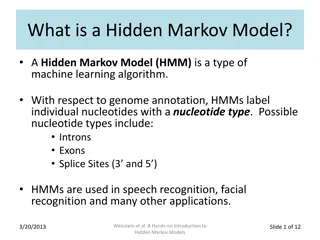
Hidden MM Uses Part of speech tagging Speech recognition Gene sequencing
Hidden Markov Model (HMM) Can be used to model state sequences and observation sequences Example: P(s,w) = i P(si|si-1)P(wi|si) S0 S1 S2 S3 Sn W1 W2 W3 Wn
Generative Algorithm Pick start state from For t = 1..T Move to another state based on A Emit an observation based on B
State Transition Probabilities start 0.2 G H 0.8 0.4 0.6
Emission Probabilities P(Ot=k|Xt=si,Xt+1=sj) = bijk x y z G H 0.7 0.2 0.1 0.3 0.5 0.2
All Parameters of the Model Initial P(G|start) = 1.0, P(H|start) = 0.0 Transition P(G|G) = 0.8, P(G|H) = 0.6, P(H|G) = 0.2, P(H|H) = 0.4 Emission P(x|G) = 0.7, P(y|G) = 0.2, P(z|G) = 0.1 P(x|H) = 0.3, P(y|H) = 0.5, P(z|H) = 0.2
Observation sequence yz Starting in state G (or H), P(yz) = ? Possible sequences of states: GG GH HG HH P(yz) = P(yz|GG) + P(yz|GH) + P(yz|HG) + P(yz|HH) = = .8 x .2 x .8 x .1 + .8 x .2 x .2 x .2 + .2 x .5 x .4 x .2 + .2 x .5 x .6 x .1 = .0128+.0064+.0080+.0060 =.0332
States and Transitions An HMM is essentially a weighted finite-state transducer The states encode the most recent history The transitions encode likely sequences of states e.g., Adj-Noun or Noun-Verb or perhaps Art-Adj-Noun Use MLE to estimate the probabilities Another way to think of an HMM It s a natural extension of Na ve Bayes to sequences
Emissions Estimating the emission probabilities Harder than transition probabilities There may be novel uses of word/POS combinations Suggestions It is possible to use standard smoothing As well as heuristics (e.g., based on the spelling of the words)
Sequence of Observations The observer can only see the emitted symbols Observation likelihood Given the observation sequence S and the model = (A,B, ), what is the probability P(S| ) that the sequence was generated by that model. Being able to compute the probability of the observations sequence turns the HMM into a language model
Tasks with HMM Given = (A,B, ), find P(O| ) Uses the Forward Algorithm Given O, , find (X1, XT+1) Uses the Viterbi Algorithm Given O and a space of all possible 1..m, find model i that best describes the observations Uses Expectation-Maximization
Inference Find the most likely sequence of tags, given the sequence of words t* = argmaxt P(t|w) Given the model , it is possible to compute P (t|w) for all values of t In practice, there are way too many combinations Greedy Search Beam Search One possible solution Uses partial hypotheses At each state, only keep the k best hypotheses so far May not work
Viterbi Algorithm Find the best path up to observation i and state s Characteristics Uses dynamic programming Memoization Backpointers
HMM Trellis end end end end P(y|G) G G G G P(H|G) P(H|H) H H H H start start start start
HMM Trellis end end end end P(G,t=1) = P(start) x P(G|start) x P(y|G) P(G,t=1) G G G G H H H H start start start start y . z
HMM Trellis end end end end P(H,t=1) = P(start) x P(H|start) x P(y|H) G G G G P(H,t=1) H H H H start start start start y . z
HMM Trellis end end end end P(H,t=2) = max (P(G,t=1) x P(H|G) x P(z|H), P(H,t=1) x P(H|H) x P(z|H)) G G G G P(H,t=2) H H H H start start start start y . z
HMM Trellis end end end end G G G G P(H,t=2) H H H H start start start start y . z
HMM Trellis end end end end G G G G H H H H start start start start y . z
HMM Trellis P(end,t=3) end end end end G G G G H H H H start start start start y . z
HMM Trellis P(end,t=3) end end end end P(end,t=3) = max (P(G,t=2) x P(end|G), P(H,t=2) x P(end|H)) G G G G H H H H start start start start y . z
HMM Trellis P(end,t=3) end end end end P(end,t=3) = max (P(G,t=2) x P(end|G), P(H,t=2) x P(end|H)) G G G G P(end,t=3) = best score for the sequence Use the backpointers to find the sequence of states. H H H H start start start start y . z
Some Observations Advantages of HMMs Relatively high accuracy Easy to train Higher-Order HMM The previous example was about bigram HMMs How can you modify it to work with trigrams?
How to compute P(O) Viterbi was used to find the most likely sequence of states that matches the observation What if we want to find all sequences that match the observation We can add their probabilities (because they are mutually exclusive) to form the probability of the observation This is done using the Forward Algorithm
The Forward Algorithm Very similar to Viterbi Instead of max we use sum Source: Wikipedia


")


")