Key Distinctions in Learning Bayesian Networks

In this tutorial from UAI 1999, important concepts in learning Bayesian networks are explored, such as complete vs. incomplete data, observed vs. hidden variables, parameters vs. structure learning, and more. The lecture covers an introduction to Bayesian statistics, learning parameters of Bayesian networks, and the Maximum Likelihood approach for optimizing data probabilities. It also discusses natural estimates, a priori ideas, and generalizing to a dice with 6 sides. Dive into these foundational topics to deepen your understanding of machine learning and research methodologies.

Download Presentation

Please find below an Image/Link to download the presentation.
The content on the website is provided AS IS for your information and personal use only. It may not be sold, licensed, or shared on other websites without obtaining consent from the author.If you encounter any issues during the download, it is possible that the publisher has removed the file from their server.
You are allowed to download the files provided on this website for personal or commercial use, subject to the condition that they are used lawfully. All files are the property of their respective owners.
The content on the website is provided AS IS for your information and personal use only. It may not be sold, licensed, or shared on other websites without obtaining consent from the author.
E N D
Presentation Transcript
White Parts from: Technical overview for machine-learning researcher slides from UAI 1999 tutorial 1
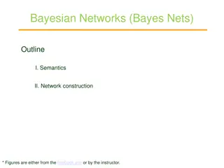
Important Distinctions in Learning BNs Complete data versus incomplete data Observed variables versus hidden variables Learning parameters versus learning structure Scoring methods versus conditional independence tests methods Exact scores versus asymptotic scores Search strategies versus Optimal learning of trees/polytrees/TANs 2
Overview of todays lecture Introduction to Bayesian statistics Learning parameters of Bayesian networks The lecture today assumes: complete data, observable variables, no hidden variables. 3
Maximum Likelihood approach: maximize probability of data with respect to the unknown parameter(s). Likelihood function: P(hhth ttth)= #h(1- )#t = A(1- )B Equivalent method is to maximize the log-likelihood function. The maximum for such sampling data is obtained when = A/ (A + B) 4
What if #heads is zero ? The maximum for such sampling data is obtained when = A / (A+B) = 0 A regularized maximum likelihood solution is needed When the data is small . = A+ / (A+B+2 ) where is some small number. What is the meaning of aside of a needed correction? 5
What if we have some idea a priori? If our a priori idea is equivalent to seeing a heads, and b tails and now we see data of A heads and B tails, then what is a natural estimate for ? If we use the estimate = a/( a+b ) as a prior guess, then after seeing the data our natural estimate changes to: = ( A+a )/(N+N ) where N = a+b, N =A+B. So what is a good choice for {a, b} ? For a random coin, maybe (100,100)? For a random thumbtack maybe (7,3)? a and b are imaginary counts, N= a+b is the equivalent sample size while A, B are the data counts and A+B is the data size. What is the meaning of in the previous slide ? 6
Generalizing to a Dice with 6 sides If our a priori idea is equivalent to seeing a1, ,a6 counts from each state and we now see data A1 A6 counts from each state, then what is a natural estimate for ? If we use a point estimate = (a1/N, ,an/N) then after seeing the data our point estimate changes to =( ( a1+A1)/(N+N ), ,(an+An)/(N+N )) Note that posterior estimate can be updated after each data point (namely in sequel or online ) and that the posterior can serve as prior for future data points. 7
Another view of the update We just saw that from = (a1/N, ,an/N) we move on after seeing the data to i = ( ai+Ai)/(N+N ) for each i. This update can be viewed as a weighted mixture of prior knowledge with data estimates: i = N/(N+N ) (ai/N) + N /(N+N ) (Ai/N ) 8
The Full Bayesian Approach Use a priori knowledge about the parameters. Encode uncertainty about the parameters via a distribution. Update the distribution after data is seen. Choose expected value as estimate. 9
(As before) p( |data) = p( ) p(data| ) 10
If we had more 100 heads the peak would move much more to the right. If we had 50 heads and 50 tails the peak would just sharpen considerably. p( |data) = p( | hhth ttth) = p( ) p( hhth ttth| ) p( | data) = p( ) #h (1- ) #t = p( | #h, #t) (#h, #t) are sufficient statistics for binomial sampling 11
The Beta distribution as a prior for =f 12
The Beta prior distribution for Example: ht htthh 16
From Prior to Posterior Observation 1: If the prior is Beta( ;a,b) and we have seen A heads and B tails, then the posterior is Beta( ;A+a,B+b). Consequence: If the prior is Beta( ;a,b) and we use a point estimate = a/N, then after seeing the data our point estimate changes to = (A+a)/(N+N ) where N =A+B. So what is a good choice for the hyper-parameters {a, b} ? For a random coin, maybe (100,100)? For a random thumbtack maybe (7,3)? a and b are imaginary counts, N=a+b is the equivalent sample size while A, B are the data counts and A+B is the data size. 19
From Prior to Posterior in Blocks Observation 2: If the prior is Dir(a1, ,an) and we have seen A1 An counts from each state, then the posterior is Dir(a1+A1, , an+An). Consequence: If the prior is Dir(a1, ,an) and we use a point estimate = (a1/N, ,an/N) then after seeing the data our point estimate changes to =( ( a1+A1)/(N+N ), ,(an+An)/(N+N )) Note that posterior distribution can be updated after each data point (namely in sequel or online ) and that the posterior can serve as prior for the future data points. 24
Another view of the update Recall the Consequence that from = (a1/N, ,an/N) we move on after seeing the data to i = ( ai+Ai)/(N+N ) for each i. This update can be viewed as mixture of prior and data estimates: i = N/(N+N ) (ai/N) + N (N+N ) (Ai/N ) 25
Learning Bayes Net parameters with complete data no hidden variables 27
Learning Bayes Net parameters p( ), p(h| ) = and p(t| ) = 1- 28
P(X=x | x) = x P(Y=y |X=x, y|x, y|~x)= y|x P(Y=y |X=~x, y|x, y|~x)= y|~x Global and Local parameter independence three separate independent thumbtack estimation tasks, assuming complete data. 30


")


 = x")