Liénard-Wiechert Results and Energy Density in Electrodynamics
Delve into the Liénard-Wiechert results and explore topics such as energy density and flux associated with electromagnetic fields. Understand the solutions of Maxwell's equations in the Lorentz gauge, focusing on the determination of scalar and vector potentials for moving point particles. Examine the fields produced by a point charge moving along a trajectory and unravel the complexities of potential functions in this context.

Download Presentation

Please find below an Image/Link to download the presentation.
The content on the website is provided AS IS for your information and personal use only. It may not be sold, licensed, or shared on other websites without obtaining consent from the author.If you encounter any issues during the download, it is possible that the publisher has removed the file from their server.
You are allowed to download the files provided on this website for personal or commercial use, subject to the condition that they are used lawfully. All files are the property of their respective owners.
The content on the website is provided AS IS for your information and personal use only. It may not be sold, licensed, or shared on other websites without obtaining consent from the author.
E N D
Presentation Transcript
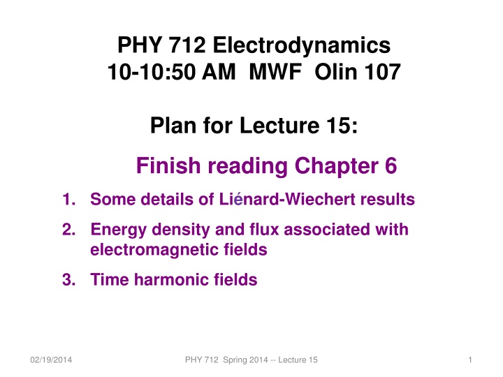
PHY 712 Electrodynamics 10-10:50 AM MWF Olin 107 Plan for Lecture 15: Finish reading Chapter 6 1. Some details of Li nard-Wiechert results 2. Energy density and flux associated with electromagnetic fields 3. Time harmonic fields 02/19/2014 PHY 712 Spring 2014 -- Lecture 15 1
02/19/2014 PHY 712 Spring 2014 -- Lecture 15 2
02/19/2014 PHY 712 Spring 2014 -- Lecture 15 3
02/19/2014 PHY 712 Spring 2014 -- Lecture 15 4
Solution of Maxwells equations in the Lorentz gauge -- continued Li nard-Wiechert potentials and fields -- Determination of the scalar and vector potentials for a moving point particle (also see Landau and Lifshitz The Classical Theory of Fields, Chapter 8.) Consider the fields produced by the following source: a point charge q moving on a trajectory Rq(t). = 3 r r R Charge density: ( , ) t ( ( )) t q q R ( ) t d q = 3 J r R r R R Current density: ( , ) ( ) t ( ( )), where t ( ) t . t q q q q dt Rq(t) q 02/19/2014 PHY 712 Spring 2014 -- Lecture 15 5
Solution of Maxwells equations in the Lorentz gauge -- continued ( , ' ') r r r 1 t ( ) = 3 ( , ) r r r d r dt ' ' ' ( | ' | / ) c t t t 4 | '] | 0 J r 1 ( ',t') r r ( ) = ' ( 3 ( , ) A r r r d r dt d r ] ' 3' | '| / ) . c t t t 2 4 | '| c 0 We performing the integrations over first d3r and then dt making use of the fact that for any function of t , ( ( ) ( | ( )| / ) ' ' ' q d f t t t t t ( ) r f t r ) = r R ' , c R r R R ( ) ( | c ( )) )| t t q r q r 1 ( t q r where the ``retarded time'' is defined to be | r t t r R ( )|. t q r c 02/19/2014 PHY 712 Spring 2014 -- Lecture 15 6
Comment on Lienard-Wiechert potential results function any for that Note : F(x) Now = ( ) ( ) ( ) F x x x dx F x 0 0 - = = consider function a for which , for 0 , 2 , 1 p(x) p(x ) i i dp ( ) i - - = ( ) ( ( )) ( ) F x p x dx F x x x dx x i dx x i ( ) F i = i dp dx x i 02/19/2014 PHY 712 Spring 2014 -- Lecture 15 7
Comment on Lienard-Wiechert potential results -- continued ( ) ( R f t ( ) = r In this case we have: ( ') f t ( ') p t ' dt ) ( ) r t c ( ) t R r R ' - q q 1 ( ) r t r q ( ) t r R ' q where: ( ') ' p t t t c ( ) ' c R ' d t ( ) ( ) t ( ) q r R ( ) t c ( ) t ' R r R ' ' ( ') ' dt dp t q dt q q = 1 1 ( ) t ( ) t r R r R ' ' q q 02/19/2014 PHY 712 Spring 2014 -- Lecture 15 8
Solution of Maxwells equations in the Lorentz gauge -- continued Resulting scalar and vector potentials: 1 q = ( , ) r , t v R 4 R 0 c v v R q = A ( , r ) , t 2 4 c R 0 c Notation: R r R ( ) rt r R | ( )|. t q q r t t r v R ( ), c rt q 02/19/2014 PHY 712 Spring 2014 -- Lecture 15 9
Solution of Maxwells equations in the Lorentz gauge -- continued In order to find the electric and magnetic fields, we need to evaluate ( , ) ( , ) t t = r r E A r ( , ) t t = A r ( , ) B r ( , ) t t The trick of evaluating these derivatives is that the retarded time trdepends on position r and on itself. We can show the following results using the shorthand notation: rt t R v R R = . = rt and c R v R R c c 02/19/2014 PHY 712 Spring 2014 -- Lecture 15 10
Solution of Maxwells equations in the Lorentz gauge -- continued 2 v R v R 1 v v c q v c = + ( , r R R ) 1 , t R 3 2 2 4 c c R 0 R c 2 A r v v R v v v R ( , ) t 1 v R t q R v c R R = . R 3 2 2 2 4 c Rc c c c 0 R c 2 v v v 1 v q R c v c R c = + E ( , ) r R R R 1 . t 3 2 2 4 c R 0 R c R v v 2 v R R v R E r / ( , ) cR q v c c t = + = B r ( , ) t 1 3 2 2 2 2 4 c c R v R 0 R R c c 02/19/2014 PHY 712 Spring 2014 -- Lecture 15 11
= D Coulomb' law s : free D t = H J Ampere - Maxwell' law s : free B t + = E Faraday' law s : 0 = B magnetic No monopoles : 0 Energy analysis of electromagnetic fields and sources source on done work of Rate J r , electromag by netic field : ( t) dE dW = 3 E J mech d r dt dt Expressing source current in terms of produces it fields : D dW = 3 E H d r dt t 02/19/2014 PHY 712 Spring 2014 -- Lecture 15 12
Energy analysis of electromagnetic fields and sources - - continued dt D t dW = = 3 3 E J E H d r d r D t B t ( ) = + + 3 E H E H d r S E 1 H Let " Poynting vector" ( ) + E D H B energy density u 2 u + = S E J t 02/19/2014 PHY 712 Spring 2014 -- Lecture 15 13
Energy analysis of electromagnetic fields and sources - - continued dt dE 3 E J mech d r 1 ( ) + E D H B Electromag netic energy density : u 2 ( ) 3 r , E d r u t field S E H Poynting vector : u + = S E J previous the From energy analysis : t dE dE ( ) ( ) PHY 712 Spring 2014 -- Lecture 15 field + = = 3 2 r S r S r , , mech d r t d r t dt dt 02/19/2014 14
Momentum analysis of electromagnetic fields and sources ( + analogy wi by Follows q F P dt d ) 3 E J B mech d r Lorentz th force : ( ) = + E v B ( ) = 3 P E B d r 0 field Expression for vacuum d field fields : P dt T P dt d j Maxwell ij + = 3 mech d r r j i stress tensor : ( ) 1 + + 2 2 E E B B T E E c B B c 0 ij i j i j ij 2 02/19/2014 PHY 712 Spring 2014 -- Lecture 15 15
Comment on treatment of time-harmonic fields ansformati Fourier tr in time on domain : 1 ~ E = i t E ,t) r r e ( d ( , ) 2 ~ E ( = i t r E r e ( , ) dt ( ,t) ~ ~ = * E r E r E r Note that is real ,t) ( , ) ( , ) These relations notion the and of superposit the principle, ion common tre the to lead atment : ( ) ( ) 1 ~ ~ ~ = + * i t i t i t E r E r E r E r ( ,t) ( , )e ( , )e ( , )e 2 02/19/2014 PHY 712 Spring 2014 -- Lecture 15 16
Comment on treatment of time-harmonic fields -- continued Equations for time harmonic fields : ( ) ( ) 1 ~ ~ ~ = + * i t i t i t E r E r E r E r ( ,t) ( , )e ( , )e ( , )e 2 ~ D ~ = = D Coulomb' law s : free free D t ~ H ~ D ~ J = + i = H J Ampere - Maxwell' law s : free free B t ~ E ~ B + = i = E Faraday' law s : 0 0 ~ B = = B magnetic No monopoles : 0 0 Note -- in all of these, the real part is taken at the end of the calculation. 02/19/2014 PHY 712 Spring 2014 -- Lecture 15 17
Comment on treatment of time-harmonic fields -- continued Equations for time harmonic fields : ( ) ( ) 1 ~ ~ ~ = + * i t i t i t E r E r E r E r ( ,t) ( , )e ( , )e ( , )e 2 ,t) ( ) ,t r = S E r H r Poynting vector : ( ( ,t) ~ ( ( ) ( ) 1 ~ ~ ~ ( ) ,t r = + + * * i t i t i t i t S E r E r H r H r ( , )e ( , )e ( , )e ( , )e 4 ) 1 ~ ~ ~ ~ = + * * E r H r E r H r ( , ) ( , ) ( , ) ( , ) 4 ( ) 1 ~ ~ ~ ~ + + 2 * * 2 i t i t E r H r E r H r ( , ) ( , )e ( , ) ( , )e 4 ( ) 1 ~ ~ ( ) ,t r = * S E r H r ( , ) ( , ) avg 2 t 02/19/2014 PHY 712 Spring 2014 -- Lecture 15 18
02/19/2014 PHY 712 Spring 2014 -- Lecture 15 19
Summary and review = D Coulomb' law s : free D t = H J Ampere - Maxwell' law s : free B t + = E Faraday' law s : 0 = B magnetic No monopoles : 0 02/19/2014 PHY 712 Spring 2014 -- Lecture 15 20
= = D E B H For linear isotropic media - - ; sources no and : = E Coulomb' law s : 0 E t = B Ampere - Maxwell' law s : 0 B t + = E Faraday' law s : 0 = B magnetic No monopoles : 0 02/19/2014 PHY 712 Spring 2014 -- Lecture 15 21
Analysis of Maxwells equations without sources -- continued: : law s Coulomb' E = 0 E t = B Ampere - Maxwell' law s : 0 B t + = E Faraday' law s : 0 = B magnetic No monopoles : 0 ( ) t E E = 2 B B t 2 B = + = 2 B 0 2 t ) ( t B B + = + 2 E E t 2 E = + = 2 E 0 2 t 02/19/2014 PHY 712 Spring 2014 -- Lecture 15 22
Analysis of Maxwells equations without sources -- continued: Both E and B fields are solutions to a wave equation: 2 B 1 v = 2 B 0 2 2 t 2 E 1 v = 2 E 0 2 2 t 2 c 2 2 0 0 where v c wave to 2 n equation Plane wave solutions : ( ) ( ) ( ) ( ) = = k r k r i i t i i t B r B E r E , , t e t e 0 0 02/19/2014 PHY 712 Spring 2014 -- Lecture 15 23
Analysis of Maxwells equations without sources -- continued: wave to solutions wave Plane = e t B r B equation = t r : ( ) ( ) ( ) ( ) i i k r k r i t i t E E , , e 0 0 2 2 v c n 2 = = k where n 0 0 Note: , n, k can all be complex; for the moment we will assume that they are all real (no dissipation). E B Note that and independen not are t; 0 0 B t + = E from Faraday' law s : 0 k c k E E n = = B 0 0 0 k k = = E B also note : and 0 0 0 0 02/19/2014 PHY 712 Spring 2014 -- Lecture 15 24
Analysis of Maxwells equations without sources -- continued: electromag plane of Summary c v electromag plane for vector Poynting netic waves : k c ( ) E n ( ) ( ) i i = = k r k r i t i t B r E r E 0 , , t e t e 0 2 2 n k 2 = = = k E where and 0 n 0 0 0 netic waves : * k c E 1 1 n i i = k r k r i t i t S E 0 e e 0 2 avg 2 E 2 n 1 k k 2 0 c = = E 0 2 02/19/2014 PHY 712 Spring 2014 -- Lecture 15 25
Analysis of Maxwells equations without sources -- continued: electromag plane of Summary c v electromag plane for density Energy netic waves : k c ( ) E n ( ) ( ) i i = = k r k r i t i t B r E r E 0 , , t e t e 0 2 2 n k 2 = = = k E where and 0 n 0 0 0 netic waves : ( ) ( ) 1 * i i = + k r k r i t i t E E u e e 0 0 4 avg * k k c c E E 1 1 n n i i k r k r i t i t 0 0 e e 4 1 2 = E 02/19/2014 0 2 PHY 712 Spring 2014 -- Lecture 15 26