Physics 301 Lecture 13: Fourier Transforms and Integral Transformations

PHYSICS 301 Lecture 13 Fourier Transforms

Introduction-a Frequently in mathematical physics we encounter pairs of functions related by an expression of the following form: ( ) ( ) ( , ) g f t K a = b a t dt a ( ) ( ) g a f t The function is called the integral transform of by the kernel . ( , ) K t a

Introduction-b Examples of integral transforms Integral Transforms Fourier Kernel Form + - - iat ( ) f t e dt iat e + - Laplace - at ( ) f t e dt e- at + - + - 1 2 Hankel ( ) at ( ) a tJ ( ) f t tJ t dt n n p ta- 1 a - Mellin 1 ( ) f t t dt

Introduction-c Linearity All these transforms are linear; that is [ 1 1 2 ( ) a b ] + ( , ) a = ( ) c f t c f t K t dt 2 b b a + a ( ) ( , ) ( ) ( , ) c f t K 1 1 c f t K t dt t dt 2 2 a a b b ( ) ( , ) c f t K a = a ( ) ( , ) cf t K t dt t dt a a

Introduction-c The inverse operator If we adopt for our linear integral transformation the operator L, we obtain ( ) a = ( ) g Lf t For all the above transforms we have an inverse operator such that 1 L- - = 1 ( ) ( ) f t L g a

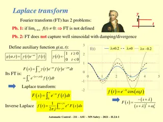
The Fourier Transform The problem that a Fourier transform answers is the representation of a non-periodic function over the infinite range. A physical example of this is the resolution of a wave packet into sinusoidal waves. The Fourier transform is defined by + [ ] = - i t w ( ) w = ( ) ( ) g F f t f t e dt - + 1 p [ ] ( ) w - i t w = ( ) w = w 1 ( ) f t F g g e d 2 -

The Fourier Transform The cosine transform If the function is even it may be represented by the so called Fourier cosine transform. + ( ) = 2 gc(w) = F f (t) f (t)cos wt dt 0 + 1 p [ ] ( ) w ( ) w = - = ( ) w w 1 ( ) cos f t F g g t d c c 0

The Fourier Transform The sine transform If the function is odd it may be represented by the so called Fourier sine transform. + ( ) = 2 gs(w) = F f (t) f (t)sin wt dt 0 + =1 gsw ( )sin wx ( ) f (x) = F-1gs(w) dw p 0

g(t - t0) g(t)eiw0t g(at) g(-t) g t ( )(t) n g(x)dx - g(t)dt = G(0) = 0 (If ) -

The Fourier Transform In three dimensional space When we move to three dimensional space the Fourier transform becomes: = - 3 i k r ( ) k ( ) r g f e d x 1 = 3 i k r ( ) f x ( ) k g e d k ( ) 2 p 3

The Fourier Transform The convolution theorem-a Some times in the probability theory we need to determine the probability density of two random independent variables f and g. This is given by the so called convolution of the functions; f t ( )*g t ( ) f x ( )g t - x ( ) dt - ( ) f t ( ) ( ) ( ) ( ) ( ) ( ) ( ) ( ) ( ) * = * * , * = * * g t g t f t f t f t f t f t f t f t 1 2 3 1 2 3 ( ) ( ) ( ) ( ) ( ) ( ) ( ) + + * = * * f t f t f t f t f t f t f t 1 2 3 1 2 1 3

The Fourier Transform The convolution theorem-b Let s assume that J( ) and G( ) are the Fourier transforms of the functions j(t) and g(t). It can be proved that the Fourier inverse transform of a product of Fourier transforms is the convolution of the original functions [ ] ( ) ( ) G w ( ) ( ) G w * = w - w = * 1 ( ) ( ) F j t g t J ( ) j t ( ) F J g t

The Fourier Transform The frequency convolution theorem F w 2( ) 1( ) f t 1( ) f t Let the functions , with Fourier transforms , . We can prove the frequency convolution theorem: ) F w 2( ( ) w ( ) w - = ( ) ( ) f t f t p ( ) 1 * 2 F F F 1 2 1 2 F w Let s assume that It can be proved is the Fourier transform of the function f . 1 p ( ) ( ) w 2 2 = w f t dt F d 2 - -

The Fourier Transform The momentum representation-a ( ) x y In quantum mechanics the wave function, , which is a solution of Schr dinger equation, has the following properties: 1. is the probability of finding the particle between x and x+dx. 2. ( ) ( ) 1 x x dx y y - ( ) ( ) y y *x x dx + = * 3. + ( ) x x ( ) x dx y = y * x -

The Fourier Transform The momentum representation-b ( ) g p We want a function. , that will give the same information for momentum: 1. is the probability of finding the particle with momentum between p and p+dp. 2. ( ) ( ) 1 g p g p dp - ( ) ( ) p g p dp * g + = * 3. + ( ) p pg p dp ( ) = * p g -

The Fourier Transform The momentum representation-c Such a function is given by the Fourier transform of our space function , ( ) x y The corresponding three-dimensional momentum function is

Mathematical Supplement The Dirac Delta function -a The Dirac function in the one-dimensional case is defined as: d = ( ) 0, 0 x x ( ) x dx d - ( ) ( ) f x d = = 1, (0) x dx f -

Mathematical Supplement The Dirac Delta function -b Delta function has also the following properties: 1 a x ( ) ( ) d - = d - , a x x x x 1 1 ( )( ) ( ) ( ) d - - = d - + d - - / x x x x x x x x x 1 2 1 2 1 2 xdd x ( ) dx = -d x ( ), d'x ( ) f (x)dx = - f'(0) - F d t ( ) ( ) =1, F(eiw0t) = 2pd w -w0

The Fourier Transform of a periodic function Periodic functions can also be Fourier transformed. We can show that if g(t) is a periodic function with period T then its Fourier transform is given by cn ( ) F(w) = 2p d w - nw0 cn n=-w Where the coefficients are associated with the corresponding Fourier series representation of the function

Mathematical Supplement Tables of Fourier transforms In the literature we can find tables with Fourier transforms of different functions. We give here such a table which also contains useful trigonometric formulae and integrals. (Click here).