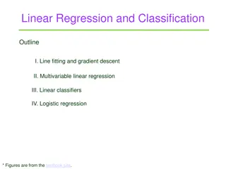
Regression Through Gradient Descent Optimization

Classification and Prediction: Regression Via Gradient Descent Optimization Bamshad Mobasher DePaul University

Linear Regression Linear regression: involves a response variable y and a single predictor variable x The weights w0 (y-intercept) and w1 (slope) are regression coefficients Method of least squares: estimates the best-fitting straight line w0 and w1 are obtained by minimizing the sum of the squared errors (a.k.a. residuals) 2 ( i i y = y = w0 + w1 x = 2 y ) e y i i i + 2 ( ( )) w w x 0 1 i i w1 can be obtained by setting the partial derivative of the SSE to 0 and solving for w1, ultimately resulting in: i ( )( ) x x y y = i i w = w y w x i 0 1 1 2 ( ) x x i 2

Multiple Linear Regression Multiple linear regression: involves more than one predictor variable Features represented as x1, x2, , xd Training data is of the form (x1, y1), (x2, y2), , (xn, yn) (each xj is a row vector in matrix X, i.e. a row in the data) For a specific value of a feature xi in data item xj we use: Ex. For 2-D data, the regression function is: x1 j ix = + + y w w x w x 0 1 1 2 2 y x2 d = i = = + = + T w . x y ( ,..., ) f x x w w x w More generally: 1 0 0 d i i 1 3

Least Squares Generalization Multiple dimensions To simplify add a new feature x0 = 1 to feature vector x: x1 x0 x2 y 1 1 1 1 1 d d = i = i = = + = = T w . x y ( , ,..., ) f x x x w x w x w x 0 1 0 0 d i i i i 1 0

Least Squares Generalization d d = i = i = = = + = = T x w x . y ( , ,..., ) ( ) f x x x f w x w x w x 0 1 0 0 d i i i i 1 0 Calculate the error function (SSE) and determine w: 2 d n d ( ) = i = j = i 2 = = = 2 i j w y x y ( ) ( ) ( ) E f w x y w x i i i i 0 1 0 = T y Xw y Xw ( ) ( = ) j y vector of training all responses y = j X x = matrix of training all samples T 1 T w X = X X y for test ( ) Closed form solution to w wE test test test w x x y sample = ( ) 0

Gradient Descent Optimization Linear regression can also be solved using Gradient Decent optimization approach GD can be used in a variety of settings to find the minimum value of functions (including non-linear functions) where a closed form solution is not available or not easily obtained Basic idea: Given an objective function J(w) (e.g., sum of squared errors), with w as a vector of variables w0, w1, , wd, iteratively minimize J(w) by finding the gradient of the function surface in the variable-space and adjusting the weights in the opposite direction The gradient is a vector with each element representing the slope of the function in the direction of one of the variables Each element is the partial derivative of function with respect to one of variables w w w ( ) ( ) ( ) f f f = = w ( ) ( , , , ) J J w w w 1 2 d w w w 1 2 d 6

Optimization An example - quadratic function in 2 variables: f( x ) = f( x1, x2 ) = x12 + x1x2 + 3x22 f( x ) is minimum where gradient of f( x ) is zero in all directions

Optimization Gradient is a vector Each element is the slope of function along direction of one of variables Each element is the partial derivative of function with respect to one of variables Example: 2 2 = = + + x ( ) ( , ) 3 f f x x x x x x 1 f 2 ) 1 f 1 2 2 x x ( x ( x ) = = = + + x ( ) ( , ) 2 6 f f x x x x x x 1 2 1 2 1 2 1 2

Optimization Gradient vector points in direction of steepest ascent of function ( , ) f 1x x 2 ( , ) ( , ) f x x x f x x x 1 2 2 1 2 1 ( , ) f 1x x 2

Optimization This two-variable example is still simple enough that we can find minimum directly 2 2 = + + ( x , x ) = 3 + f x x x x x x 1 , 2 ) 1 x 1 2 2 6 + ( 2 f x x x 1 2 1 2 1 2 Set both elements of gradient to 0 Gives two linear equations in two variables Solve for x1, x2 + = + = 2 0 6 0 x x x x 1 2 1 2 = = 0 0 x x 1 2

Optimization Finding minimum directly by closed form analytical solution often difficult or impossible Quadratic functions in many variables system of equations for partial derivatives may be ill-conditioned example: linear least squares fit where redundancy among features is high Other convex functions global minimum exists, but there is no closed form solution example: maximum likelihood solution for logistic regression Nonlinear functions partial derivatives are not linear example: f( x1, x2 ) = x1( sin( x1x2 ) ) + x22 example: sum of transfer functions in neural networks

Gradient descent optimization Given an objective (e.g., error) function E(w) = E(w0, w1, , wd) Process (follow the gradient downhill): Pick an initial set of weights (random): Determine the descent direction: Choose a learning rate: Update your position: 5. Repeat from 2) until stopping criterion is satisfied Typical stopping criteria E( wt+1 ) ~ 0 some validation metric is optimized w = (w0, w1, , wd) - E(wt) wt+1 = wt - E(wt) 1. 2. 3. 4. Note: this step involves simultaneous updating of each weight wi

Gradient descent optimization 2 d = i In Least Squares Regression: = = T 2 w y y w x ( ) ( . ) E ix w i 0 Process (follow the gradient downhill): Select initial w = (w0, w1, , wd) 2. Compute - E(w) Set Update:w := w - E(w) 5. Repeat until E( wt+1 ) ~ 0 1. 3. 1 n = 4. = T i i i j w x : ( . ) w w y x j j 2 n 1 i = for 1 , 0 ,..., j d

Illustration of Gradient Descent E(w) w1 w0

Illustration of Gradient Descent E(w) w1 w0

Illustration of Gradient Descent E(w) w1 Direction of steepest descent = direction of negative gradient w0

Illustration of Gradient Descent E(w) w1 Original point in weight space New point in weight space w0

Gradient descent optimization Problems: Choosing step size (learning rate) too small convergence is slow and inefficient too large may not converge Can get stuck on flat areas of function Easily trapped in local minima

Stochastic gradient descent Application to training a machine learning model: 1. Choose one sample from training set: xi 2. Calculate objective function for that single sample: 3. Calculate gradient from objective function: 4. Update model parameters a single step based on gradient and learning rate: T 2 i i w x ( . ) y = = T i i i j w x : ( . ) for ,..., 0 w w y x j d j j Repeat from 1) until stopping criterion is satisfied Typically entire training set is processed multiple times before stopping Order in which samples are processed can be fixed or random. 5.