Spectrum Analysis and Signal Reconstruction in Digital Signal Processing

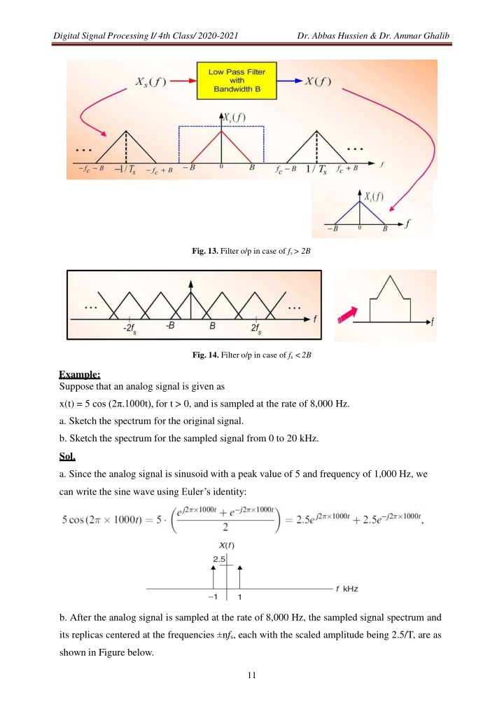
Digital Signal Processing I/ 4th Class/ 2020-2021 Dr. Abbas Hussien & Dr. Ammar Ghalib Fig. 13. Filter o/p in case of fs > 2B Fig. 14. Filter o/p in case of fs <2B Example: Suppose that an analog signal is given as x(t) = 5 cos (2 .1000t), for t > 0, and is sampled at the rate of 8,000 Hz. a. Sketch the spectrum for the original signal. b. Sketch the spectrum for the sampled signal from 0 to 20 kHz. Sol. a. Since the analog signal is sinusoid with a peak value of 5 and frequency of 1,000 Hz, we can write the sine wave using Euler s identity: b. After the analog signal is sampled at the rate of 8,000 Hz, the sampled signal spectrum and its replicas centered at the frequencies nfs, each with the scaled amplitude being 2.5/T, are as shown in Figure below. 11

Digital Signal Processing I/ 4th Class/ 2020-2021 Dr. Abbas Hussien & Dr. Ammar Ghalib Notice that the spectrum of the sampled signal contains the images of the original spectrum; that the images repeat at multiples of the sampling frequency fs(for our example, 8 kHz, 16 kHz, 24 kHz, . . . ); and that all images must be removed, since they convey no additional information. Signal reconstruction Two simplified steps are involved, as described in Fig. 15. First, the digitally processed data y(n) are converted to the ideal impulse train ys(t), in which each impulse has its amplitude proportional to digital output y(n), and two consecutive impulses are separated by a sampling period of T; second, the analog reconstruction filter is applied to the ideally recovered sampled signal ys(t) to obtain the recovered analog signal. Fig. 15. Signal notations at reconstruction stage The following three cases are listed for recovery of the original signal spectrum: Case 1: fs = 2fmax: Nyquist frequency is equal to the maximum frequency of the analog signal x(t), an ideal lowpass reconstruction filter is required to recover the analog signal spectrum. 12

Digital Signal Processing I/ 4th Class/ 2020-2021 Dr. Abbas Hussien & Dr. Ammar Ghalib This is an impractical case. Case 2: fs> 2fmax: In this case, there is a separation between the highest frequency edge of the baseband spectrum and the lower edge of the first replica. Therefore, a practical lowpass reconstruction (anti-image) filter can be designed to reject all the images and achieve the original signal spectrum. Case 3: fs< 2fmax: This is aliasing, where the recovered baseband spectrum suffers spectral distortion, that is, contains an aliasing noise spectrum; in time domain, the recovered analog signal may consist of the aliasing noise frequency or frequencies. Hence, the recovered analog signal is incurably distorted. Example: Assuming that an analog signal is given by x(t) = 5cos(2 .2000t) +3cos(2 .3000t) for t 0, and it is sampled at the rate of 8,000 Hz, a. Sketch the spectrum of the sampled signal up to 20 kHz. b. Sketch the recovered analog signal spectrum if an ideal lowpass filter with a cutoff frequency of 4 kHz is used to filter the sampled signal (y(n)=x(n) in this case) to recover the original signal. Sol. Using Euler s identity, we get a. The two-sided amplitude spectrum for the sinusoids (sampled signal) is displayed in Fig. b. Based on the spectrum in (a), the sampling theorem condition is satisfied; hence, we can recover the original spectrum using a reconstruction lowpass filter. The recovered spectrum is shown in the following Fig. Aliasing noise level Given the DSP system shown in Fig. 16, where we can find the percentage of the 13

Digital Signal Processing I/ 4th Class/ 2020-2021 Dr. Abbas Hussien & Dr. Ammar Ghalib aliasing noise level using the symmetry of the Butterworth magnitude function and its first replica. Then: Fig. 16. DSP system with anti-aliasing filter fa 2n 1+ f c Aliasing noise level %= for 0 f fc f s fa 2n 1+ fc Where, n is the filter order, fais the aliasing frequency, fcis the cutoff frequency, and fsis the sampling frequency. Example: In a DSP system with anti-aliasing filter, if a sampling rate of 8,000 Hz is used and the anti-aliasing filter is a second-order Butterworth lowpass filter with a cutoff frequency of 3.4 kHz, a. Determine the percentage of aliasing level at the cutoff frequency. b. Determine the percentage of aliasing level at the frequency of 1,000 Hz. Sol. 14