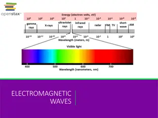
Time-Varying Fields in Maxwell's Equations

Lect.03 Time Varying Fields and Maxwell s Equations Prepared by Dr. Eng. Sherif Hekal 3/18/2025 Lecture 03 1

Introduction Important definitions Electric field intensity (V/m) ? Magnetic field intensity (A/m) Electric flux density (Coulomb/m2) ? ? Magnetic flux density (Weber/m2) or Tesla ? ? = ?0??? ? = ?0??? ?0 = Permittivity of free space = 8.85x10-12 Farad/m ?0 = Permeability of free space = 4 x10-7 Henry/m ?? = Relative Permittivity of media ?? = Relative Permeability of media 3/18/2025 Lecture 03 2

Introduction Time-Varying Fields Stationary charges electrostatic fields Steady currents magnetostatic fields Time-varying currents electromagnetic fields Only in a non-time-varying case can electric and magnetic fields be considered as independent of each other. In a time-varying (dynamic) case the two fields are interdependent. A changing magnetic field induces an electric field, and vice versa. 3 3/18/2025 Lecture 03

Sources of Electric field, magnetic field Sources of Electric field, magnetic field From Coulomb's Law, a point charge dq generates electric field distance away from the source: r dq 1 dq r P = d E r r 4 2 0 dE Ids From Biot-Savart's Law, a point current magnetic field distance away from the source: generates r dB 4 Id r s = r d B 0 2 Difference: 1. A current segment , not a point charge dq, hence a vector. 2. Cross product of two vectors, is determined by the right- hand rule. 3/18/2025 Ids Ids dB Lecture 03 4

Maxwells equations Gauss Gauss Law for Electric Field Law for Electric Field It states that The total electric flux passing through any closed surface is equal to the total charge enclosed by that surface. = Q (2.1) E enc S S = = d D d S (2.2) E E v = Q dv Total charge enclosed (2.3) enc v S v = D d S dv (2.4) v 3/18/2025 Lecture 03 5

Maxwells equations Using Divergence Theorem = D d S D dv (2.5) S v Comparing the two volume integrals in (2.4) and (2.5) = D (2.6) v This is the first Maxwell s equation. It states that the volume charge density is the same as the divergence of the electric flux density. 3/18/2025 Lecture 03 6

Maxwells equations Gauss Law for Gauss Law for Magnetic Field Magnetic Field The magnetic flux density B is related to the magnetic field intensity H = B H (2.7) 0 where o is a constant and is known as the permeability of free space. Its unit is Henry/meter (H/m) and has the value = 7 4 10 H/m 0 The magnetic flux through a surface S is given by S = B d S (2.8) m where the magnetic flux m is in webers (Wb) and the magnetic flux density is in weber/ m2 or Tesla. 3/18/2025 Lecture 03 7

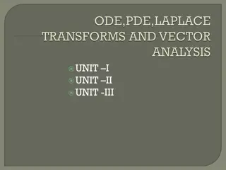
Maxwells equations Magnetic flux lines due to a straight wire with current coming out of the page Each magnetic flux line is closed with no beginning and no end and are also not crossing each other. In an electrostatic field, the flux passing through a closed surface is the same as the charge enclosed. S = = D d S Q E Thus it is possible to have an isolated electric charge. Also the electric flux lines are not necessarily closed. 3/18/2025 Lecture 03 8

Maxwells equations Magnetic flux lines are always close upon themselves,. So it is not possible to have an isolated magnetic charges. An isolated magnetic charge does not exist. Thus the total flux through a closed surface in a magnetic field must be zero. B S = 0 d S (2.9) This equation is known as the law of conservation of magnetic flux or Gauss s Law for Magnetostatic fields. 3/18/2025 Lecture 03 9

Maxwells equations Applying Divergence theorem, we get S v = = 0 B d S B dv B = 0 or (2.10) This is Maxwell s second equation. This equation suggests that magnetostatic fields have no source or sinks. Also magnetic flux lines are always continuous. 3/18/2025 Lecture 03 10

Maxwells equations Faraday s law of induction Faraday s law of induction We have learned that a constant current induces magnetic field and a constant charge (or a voltage) makes an electric field. Similar phenomena happen when currents/voltages are changing in time. The relation between the electric and magnetic field components is governed by the Faraday s law ? ? = ? ?(?) (2.11) ?? Lentz s law where ?(?) is the total time-varying magnetic flux passing through a surface.

Maxwells equations Faraday s law of Faraday s law of induction, cont d induction, cont d The terminals of the loop are separated by an infinitely small distance Therefore, we consider an individual turn of a coil (inductor) as a closed loop. At a glance: an electric current (an emf) is generated in a closed loop when any change in magnetic environment around the loop occurs (Faraday s law). When an emf is generated by a change in magnetic flux according to Faraday's Law, the polarity of the induced emf is such that it produces a current whose magnetic field opposes the change which produces it. The induced magnetic field inside any loop of wire always acts to keep the magnetic flux in the loop constant.

Maxwells equations Faraday s law of Faraday s law of induction, cont d induction, cont d The total magnetic flux passing through the loop is S = t) ( B d S (2.12) m The terminals of the loop are separated by an infinitely small distance, therefore, we assume the loop as closed. the electric potential can be expressed as L = V ) ( t E dl (2.13) Combining two last equations with (2.11) yields the integral form of Faraday s law: L S = E dl B d S (2.14) t

Maxwells equations Faraday s law of Faraday s law of induction, cont d induction, cont d Application of the Stokes stheorem to the integral form of the Faraday s law of induction leads to L S S = ( = ). E l d E d S B d S (2.15) t Equality of integrals implies an equality of integrands, therefore: B = E (2.16) t Is a differential form of the Faraday s law of induction which also is the 3rd Maxwell equation

Maxwells equations Continuity Equation Continuity Equation Electric charges in motion constitute a current. The unit of current is the ampere (A), and defined as a rate of movement of charge passing a given reference point (or crossing a given reference plane) of one coulomb per second. dQ = I (2.17) dt d S v = J d S dv (2.18) c v dt ?? conduction current density v v ( = ) v J dv dv Applying Divergence theorem, we get (2.19) c t from the principle of conservation of charges we get the equation of continuity = v J (2.20) c t

Maxwells equations Ampere s Law Ampere s Law states that the line integral of H about any closed path is exactly equal to the direct current enclosed by that path, l d = H I (2.21) enc Application of the Stokes s theorem, we get ( = ) H d S J d S (2.22) c S S H = c J (2.23)

Maxwells equations Displacement Current Displacement Current H = For static EM fields J But the divergence of the curl of a vector field is zero. So ( = = ) 0 H J (2.24) But the continuity of current requires v = 0 J (2.25) t Equation (2.24) and (2.25) are incompatible for time-varying conditions So we need to modify equation (2.23) to agree with (2.25) Add a term to equation (2.23) so that it becomes = + H J d J (2.26) where Jd is to defined and determined. 3/18/2025 Lecture 03 17

Maxwells equations Displacement Displacement Current Current, cont d , cont d Again the divergence of the curl of a vector field is zero. So ( = = + d J ) 0 H J (2.27) In order for equation (2.27) to agree with (2.25) D (2.28) = = = ( = ) v J J D d D t t t or (2.29) = Jd t Putting (2.29) in (2.26), we get D = + H J (2.30) t This is Maxwell s fourth equation (based on Ampere Circuital Law) for a time- varying field. The term ??= ?? ?? is known as displacement current density and J is the conduction current density ??= ?? . 3/18/2025 Lecture 03 18

Maxwells equations Displacement Displacement Current Current, cont d , cont d Example 1: Verify that the conduction current in the wire equals to the displacement current between the plates of the parallel plate capacitor in Figure. The voltage source supplies: Vc = V0 sin t. The conduction current in the wire is dV I C dt = = cos c CV t 0 c A d = C The capacitance of a parallel plate capacitor is: V d V d = c E The electric field between the plates: = = 0sin D E t The displacement flux density is: V sin t 0 Finally: AV D d S S S = = = = = 0 cos I J ds ds ds t I d d c t t d

Maxwells equations Displacement Displacement Current Current, cont d , cont d Example 2: Find the displacement current, the displacement charge density, and the volume charge density associated with the magnetic flux density in a vacuum: = = 0cos(2 )cos( B ) B B u x t y u x x x There is no conductors, therefore, only the displacement flux exists. u u u x y z 1 1 B D t = = = = cos(2 )sin( x ) 0 J B t y u d z x y z 0 0 0 0 0 B x The displacement flux density: B B = = = cos(2 )sin( x ) cos(2 )cos( x ) 0 0 D J dt t y u d t t y u d z z 0 0 From the Gauss s law: v = = 0 D

Maxwells equations General Forms of Maxwell General Forms of Maxwell s Equations Differential Integral s Equations Remarks Gauss Law S V = = D d s dv 1 D V V S Nonexistence of isolated magnetic charge = B = 0 B d s 0 2 B L s = = E l d B d s x E Faraday s Law 3 t t D D l d = + H J d s Ampere s circuital law = + 4 x H J t t L s In 1 and 2, S is a closed surface enclosing the volume V In 2 and 3, L is a closed path that bounds the surface S 21

Electromagnetic wave equation Wave equation is a differential equation describes the propagation of electric/magnetic field with distance and time B = E Starting from Faraday s law dt Taking curl of both sides of latter equation: B t = = = E B H t t D = = , , J E D E = + H J dt E D ( = 2 E E ) t t t 3/18/2025 Lecture 03 22

Electromagnetic wave equation 2 E E = 2 E ( ) v 2 t t General form of wave equation for electric field: 2 E E = 2 E ( ) v (2.31) 2 t t For source-free region ??= 0: 2 E E = 2 E 0 (2.32) 2 t t 3/18/2025 Lecture 03 23

Electromagnetic wave equation For free space ??= 0, = 0, ? = ?0, and ? = ?0: 2 E = 2 E (2.33) 0 0 2 t 3/18/2025 Lecture 03 24

Electromagnetic wave equation Wave equation in time Wave equation in time- -harmonic fields harmonic fields For time harmonic variation (phasor representation) = = je t ( , , , ) ( , ) ( , , ) E x y z t E r t E x y z 2 t= j , = j = 2 2 ( ) 2 t Hence, the wave equation for source-free region can be given by j + = 2 2 E E E 0 + j = 2 2 E E ( ) 0 E Lecture 03 = 2 2 E 0 3/18/2025 25

Electromagnetic wave equation = + j 2 2 ( ) = = + j j 2 + Phase shift constant = wave number (rad/m) Propagation constant (m-1) Attenuation constant (Neper/m) 3/18/2025 Lecture 03 26

Electromagnetic wave equation Solution of the wave equation Solution of the wave equation E = 2 2 E 0 2 2 2 + + E = 2 E ( ) 0 2 2 2 x y z So, we have three equations = 2 2 0 E E x x = 2 2 0 E E y y = 2 2 0 E E z z 3/18/2025 Lecture 03 27

Electromagnetic wave equation For simplicity, we assume that the electric field has one component and the propagation in Z direction E = x ) ( E z a x x 2 2 = = , 0 0 2 2 y 2 E = 2 E 0 2 z Which is homogenous 2nd order differential equation 3/18/2025 Lecture 03 28

Electromagnetic wave equation d Remember: = = ( ) y f x D dx 0 = 2 2 ( ) D = a y = = 2 2 ( ) 0 , m a m a m a 1 + 2 = m x m x y c e c e 1 2 1 2 = 2 2 ( ) 0 D = E Similarly = = 2 2 ( ) 0 , m m m 1 2 + 0 0 + = + z z ( ) E z E e E e x 3/18/2025 Lecture 03 29

Electromagnetic wave equation + j + = E E e 1 Where 0 0 Complex constant j = E E e 2 0 0 Let 1 = 2 = 0 z j z e + + 0 0 + + = z j z ( ) E z E e E e e Phasor representation For time domain representation = jwt ( , ) Re ( ) E z t E z e + + = + ( ) ( ) z j t z z j t z Re E z e + e e E t e e ) 0 0 x a + = + z z ( , ) cos( ) cos( E z t E e t E z 0 0 Backward wave Forward wave 3/18/2025 Lecture 03 30

Electromagnetic wave equation = t t + + + z z a ( , ) cos ( ) cos ( ) E z t E e z E e z 0 0 x t t + = + + z z a ( , ) cos ( ) cos ( ) E z t E e z E e z 0 0 x x a + = + + ( , ) ( ) ( ) E z t f z t f z t = where = phase velocity = wave velocity 3/18/2025 Lecture 03 31

Electromagnetic wave equation Wave length ( ): The distance between two points have the same phase or the distance travelled during each cycle. The wavelength is the distance over which the spatial phase shifts by 2 radians, assuming fixed time 2 = = 2 = z = f v f f 2 2 f v = = = = f 3/18/2025 Lecture 03 32