Understanding Fourier Theory in Seismic Processing
Explore the concepts of Fourier Theory in Seismic Processing, including temporal and spatial aliasing, Nyquist frequency, Fourier series, and transforms. Learn how signals are transformed and expanded using sine and cosine functions.

Uploaded on | 2 Views
Download Presentation

Please find below an Image/Link to download the presentation.
The content on the website is provided AS IS for your information and personal use only. It may not be sold, licensed, or shared on other websites without obtaining consent from the author. If you encounter any issues during the download, it is possible that the publisher has removed the file from their server.
You are allowed to download the files provided on this website for personal or commercial use, subject to the condition that they are used lawfully. All files are the property of their respective owners.
The content on the website is provided AS IS for your information and personal use only. It may not be sold, licensed, or shared on other websites without obtaining consent from the author.
E N D
Presentation Transcript
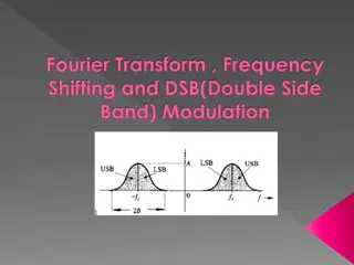
Fourier Theory in Seismic Processing (From Liner and Ikelle and Amundsen) Temporal aliasing Spatial aliasing
Also with notes from http://lcni.uoregon.edu/fft.p pt
Fourier series Periodic functions and signals may be expanded into a series of sine and cosine functions http://www.falstad.com/fourier/j2/
The Nyquist Frequency The Nyquist frequency is equal to one-half of the sampling frequency. The Nyquist frequency is the highest frequency that can be measured in a signal.
The Fourier Transform A transform takes one function (or signal) and turns it into another function (or signal)
The Fourier Transform A transform takes one function (or signal) and turns it into another function (or signal) Continuous Fourier Transform:
The Fourier Transform The input signal gives the proper weight to all the cosines and sines Continuous Fourier Transform: 2 ift ( ) ( ) h t ( ) ( ) h f e = = h f h t e dt 2 ift df
Famous Fourier Transforms 1.5 1 Sinc function 0.5 0 -0.5 -1 -0.8 -0.6 -0.4 -0.2 0 0.2 0.4 0.6 0.8 1 6 5 4 Square wave 3 2 1 0 -100 -50 0 50 100
The Fourier Transform 2 ift ( ) ( ) u t ( ) ( ) u f e = = u f u t e dt 2 ift df T 1 t 2 T = ( ) u t 0 t 2
, + 2 ift ( ) u t e = + = ( ) u f dt T 21 T i t e dt 2 ax de ax = ae dx ax e ax dx e = + k a
T i t e 2 = T i 2 T T i i 1 i 2 2 = e e 1 i T T = cos sin i 2 2 T T 1 i cos sin i 2 2
,and ie = + cos sin i i ( ) = + cos sin e i = cos sin i
1 i 1 i T T = sin sin i i 2 2 1 i 1 i T T = + sin sin i i 2 T 2 2 = sin i 2 i 2 i T = sin i 2 T sin 2 = 2 T sin 2 = 2 T sin 2 = T T 2 T = sinc T 2
Discrete Fourier Transform A transform takes one function (or signal) and turns it into another function (or signal) The Discrete Fourier Transform: 1 N H h e k n k N h H e n N k n = ikn N 2 = = 0 1 ikn N 1 2 = 0
Fast Fourier Transform The Fast Fourier Transform (FFT) is a very efficient algorithm for performing a discrete Fourier transform FFT algorithm published by Cooley & Tukey in 1965 In 1969, the 2048 point analysis of a seismic trace took 13 hours. Using the FFT, the same task on the same machine took 2.4 seconds!
A sine wave 8 5*sin (2 4t) 6 Amplitude = 5 4 Frequency = 4 Hz 2 0 -2 -4 -6 -8 0 0.1 0.2 0.3 0.4 0.5 0.6 0.7 0.8 0.9 1 seconds
A sine wave signal 8 5*sin(2 4t) 6 Amplitude = 5 4 Frequency = 4 Hz 2 Sampling rate = 256 samples/second 0 -2 Sampling duration = 1 second -4 -6 -8 0 0.1 0.2 0.3 0.4 0.5 0.6 0.7 0.8 0.9 1 seconds
An undersampled signal sin(2 8t), SR = 8.5 Hz 2 1.5 1 0.5 0 -0.5 -1 -1.5 -2 0 0.2 0.4 0.6 0.8 1 1.2 1.4 1.6 1.8 2
Sample Rates What is the fewest number of times I need to sample this waveform per second? ? ? ?
Sample Rates What is the fewest number of times I need to sample this waveform per second? At least twice per wavelength or period! OTHERWISE .
Undersampled waveforms f f Amplitude True frequency (f -true) Reconstructed frequency (f -aliased)
Oversampled waveforms Nyquist frequency Amplitude Reconstructed frequency frequency is unaliased = True frequency (f -true) Nyquist frequency = 1 / twice the sampling rate Minimum sampling rate must be at least twice the desired frequency E.g., 1000 samples per second for 500Hz, 2000 samples per second for 1000 Hz
Oversampled waveforms Nyquist frequency Amplitude In practice we are best oversampling by double the required minimum i.e. 1000 samples per second for a maximum of 500 Hz i.e., 2000 samples per second for a maximum of 1000 Hz Oversampling is relatively cheap.
Spatial aliasing Spatial frequency, or wavenumber (k) is the number of cycles per unit distance. One spatial cycle or wavenumber = frequency/velocity. Each wavenumber must be sampled at least twice per wavelength (two CMP s per wavelength) 1 = N k 2( ) CMPspacing IN PRACTICE each wavenumber must be sampled at least four times per minimum wavelength (two CMP s per wavelength)
Spatial aliasing However, dip (theta) as well as frequency and velocity event changes the number of cycles per distance, so lambda = CMPinterval Liner, 9.7,p.192 4sin
Spatial aliasing lambda = CMPinterval 4sin x V t V t = sin limit x For aliasing NOT to occur, delta(t) must be less than T/2
Spatial aliasing VT = sin limit 2 x VT = x lim it 2sin
1/4 wavelength shift per trace total shift across array=3/4 wavelength K=+ or -ve?
1/4 wavelength shift per trace total shift across array=3/4 wavelength K=?
1/2 wavelength shift per trace total shift across array=3/2 wavelength K=0
3/4 wavelength shift per trace total shift across array=2 1/4 wavelength