Understanding Ozone Trends and Analysis
Dive into the analysis of ozone trends from SBUV and OMPS-NM datasets spanning from 1979 to 2021. Explore comparisons between EPIC and OMPS, long-term ozone time series, challenges with zenith angle, and more. Discover insights on trends, turnaround dates, and regression equations to understand ozone dynamics better.

Download Presentation

Please find below an Image/Link to download the presentation.
The content on the website is provided AS IS for your information and personal use only. It may not be sold, licensed, or shared on other websites without obtaining consent from the author. If you encounter any issues during the download, it is possible that the publisher has removed the file from their server.
You are allowed to download the files provided on this website for personal or commercial use, subject to the condition that they are used lawfully. All files are the property of their respective owners.
The content on the website is provided AS IS for your information and personal use only. It may not be sold, licensed, or shared on other websites without obtaining consent from the author.
E N D
Presentation Transcript
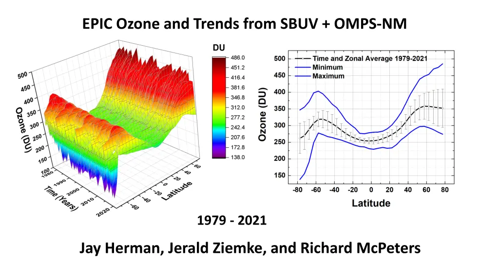
EPIC Ozone and Trends from SBUV + OMPS-NM 1979 - 2021 Jay Herman, Jerald Ziemke, and Richard McPeters
EPIC Ozone and Trends from SBUV + OMPS-NM This talk is divided in two parts 1. EPIC compared to OMPS showing good agreement for moderate SZA 2. Long-Term O3 Time Series (MOD) 1978 - 2021 Trends and Latitude Dependent Ozone Turn- Around Dates TA( ) 1994 1998 Global Models do not show this effect
EPIC vs OMPS-NM Summer values are good 65OS shows a zenith angle problem with EPIC and OMPS
Solar Zenith Angle Problem at 65S Spherical Geometry Radiative Transfer is Needed
EPIC Ozone EPIC ozone agrees well with OMPS-NPP except where there are sampling problems near the Arctic and Antarctic circles Summer values agree everywhere The EPIC data record is not long enough for trend estimation but agrees with OMPS for 2016 2022. The missing 2019 data is a problem for trend estimation.
Trends and Turnaround dates from the MOD ozone data set 1978 - 2021 MOD consists of a merged ozone data set from Nimbus 7 SBUV (1978 1990) NOAA-9 SBUV-2 NOAA-11 SBUV-2 NOAA-14 SBUV-2 NOAA-16 SBUV-2 Suomi NPP OMPS (2012 2023) NOAA-17 SBUV-2 NOAA-18 SBUV-2 NOAA-19 SBUV-1 https://acd-ext.gsfc.nasa.gov/Data_services/merged/
Multivariate Linear Regression Equations Linear trend estimates for the long-term changes in MOD(t, i) globally and as a function of latitude i have been obtained using the multivariate linear regression (MLR) model. Trends B( i) were determined for MOD(t, i) using MOD(t, i) = A( I t) + B( I,t) t + C( I,t) QBO1(t) + D( I,t) QBO2(t) + E( I,t) ENSO(t) + F( I,t) Solar(t) + R(t, I) Statistical uncertainties for the trend variables A(t) and B( i) were derived from the calculated statistical covariance matrix involving the variances and cross-covariances of the constants
Long-term trends can be calculated from deseasonalized data, either from the MLR method or from simply forming annual averages. The two methods agree closely Estimation of linear long-term trends since 1979 is misleading, since ozone showed significant annual declines until the mid- 1990s and then increased slightly thereafter, meaning the average long-term time series is non- linear. Therefore, this trend estimate is misleading
Non-Linear behavior of the Ozone time series MOD in two latitude bands and Lowess(0.3) fitting functions (f = 0.3, black lines). Examples of different f = 0.1 (Red) and 0.05 (blue dots) are shown. Note the slight downturn since 2010 in the Lowess(0.3) at 55ON.
Expanded Scale TA is from 1st derivative Lowess(0.3) fits to the MOD data for 16 latitude bands used to determine TA( ). Note that the ozone scale varies for each latitude.
A test for atmospheric models The general TA( ) pattern shown in Fig. 7 should appear in model calculations as a signature of the combined effects of photochemistry, dynamics, and volcanic eruptions on the cessation of decreasing ozone in the mid- 1990s. However, models do not show this behavior suggesting that the dynamics and chemistry are incomplete Turnaround dates TA( ) as a function of latitude
Age of Air and TA Equatorial region Dominated by upwelling Brewer Dobson circulation South Hemisphere Mid- to High-latitudes dominated by Polar Vortex winds and summer Ozone hole backfilling Northern Hemisphere Mid- to High latitudes: No Polar Vortex, No ozone hole, follows equatorial values
Ozone trends PD( ) (percent per decade) Ozone trends PD( ) (percent per decade) using the MLR and Annual Average methods before and after TA( ). 6b A magnified version of the MLR estimated trends after TA with 2 uncertainties.
Summary EPIC ozone agrees with OMPS-NM especially summer values MOD data set shows latitude dependent TA( ) Current Atmospheric Chemistry and Dynamics Models show TA = 2000 TA( ) is a useful test of 3-D Models Ability to represent Atmospheric Chemistry, Dynamics, and Volcanic Effects Herman, J., Ziemke, J., and McPeters, R.: Total Column Ozone Trends from the NASA Merged Ozone Time Series 1979 to 2021 Showing Limited Recovery to 1979 Amounts after Declining into the Mid 1990s, EGUsphere [Accepted], https://doi.org/10.5194/egusphere-2023-955, 2023.


 (percent per decade)")