Vision as Bayesian Inference and Belief Propagation

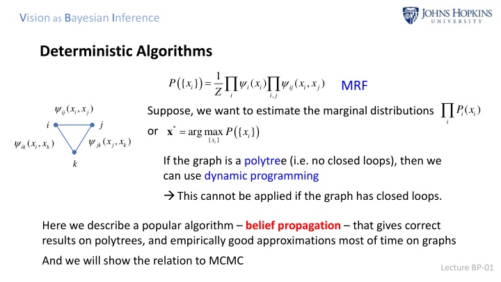
Vision as Bayesian Inference Deterministic Algorithms 1 Z = ( ) { } x ( ) x ( , x x ) P MRF i i i ij i j , i i j ( , x x ) ( ) P x Suppose, we want to estimate the marginal distributions ( ) { } i x ij i j i i i j i = * x argmax { } x P or i ( , ) x x ( , x x ) jk j k ik i k If the graph is a polytree (i.e. no closed loops), then we can use dynamic programming This cannot be applied if the graph has closed loops. k Here we describe a popular algorithm belief propagation that gives correct results on polytrees, and empirically good approximations most of time on graphs And we will show the relation to MCMC Lecture BP-01

Vision as Bayesian Inference Belief Propagation (BP) proceeds by passing messages between the graph nodes :message that node i passes to node j to affect state xj ( : ) t m x ij j The messages gets updated as follows: = + ) ( : 1) ( , x x ( ) x ( : ) m x t m x t Sum-product rule ij j ij i j i i ki i x k j i Alternative: the max-product + = ) ( : 1) max x ( , x x ( ) x ( : ) m x t m x t ij j ij i j i i ki i i k j If the algorithm converges (it may not), then we compute approximations to the marginals: ( ) ( ) ( ) i i i i ki i k ( , ) ( ) ( , ij i j i i ij i b x x x x x b x x m x ) ( ) ( ) x ( ) x m m x j j j ki i lj j Lecture BP-02 l i k j

Vision as Bayesian Inference Belief Propagation BP (sum-product) was first proposed by Judea Pearl (C.S. UCLA) for performing inference on polytrees The max-product algorithm was proposed earlier by Gallagher The application was developed in the 1990 s for decoding problems - goal was to achieve Shannon s bound on information transmission Experimentally, it was shown that BP usually converges to reasonable approximations - Full understanding of when & why it converges is an open problem On polytree, it is similar to dynamic programming so in a sense, it is the way to extend DP to graphs with closed loops Lecture BP-03

Vision as Bayesian Inference Example of BP (sum-product) = x ( , x x x x , , ) 1 2 3 4 1 2 3 4 1 Z = ) ) ( ) x ( , x x ( , x x ( , x x ) P 12 1 2 23 2 3 34 3 4 Messages: Update rule (from message passing equation) = ( : 1) ( , ) x m x t x x m ( : 1) ( , x m x t x x m ( : 1) ( , x m x t x x m ( : 1) ( , x m x t x x m ( : 1) ( , x m x t x x + boundary m12(x2), from node 1 to node 2 m21(x1), from node 2 to node 1 m23(x3), from node 2 to node 3 m32(x2), from node 3 to node 2 m34(x4), from node 3 to node 4 m43(x3), from node 4 to node 3 ( : 1) ( , x x ) m x t 12 2 12 1 2 x 1 = = = = = + ( : ) t x 21 1 12 1 2 32 2 2 + ) ( : ) t x 23 3 23 2 3 12 2 2 + ) ( : ) t x 32 2 23 2 3 43 3 3 + ) ( : ) x t 34 4 34 3 4 23 3 3 + boundary ) 43 3 34 3 4 Lecture BP-04 4

Vision as Bayesian Inference Many ways to run BP (1) Update all messages in parallel Note: BP can be parallelized but Dynamic Programming cannot) (2) Start at boundaries Then read off estimates of unary marginals 1 ( ) ( ), b x m x Z Z 1 ( ) ( ) ( b x m x m x Z 1 ( ) ( ) ( ), b x m x m x Z 1 ( ) ( ), b x m x Z Z 1 ( , ) ( , b x x x x m Z m12 m23 m34 i.e., = = ( ):normalization x m 1 2 3 4 1 1 21 1 1 21 1 m21 m32 m43 x 1 1 = ), :normalization Z 2 2 12 2 32 2 2 m12(x2), then m23(x3), then m34(x4) Forward pass (like Dynamic Programming) Calculate 2 = :normalization Z 3 3 23 3 43 3 3 m43(x3), then m32(x2), then m21(x1) Backward pass (like backward pass of DP) 3 = :normalization 4 4 34 4 4 4 = ) ( ), and so on x 12 1 2 12 1 2 32 2 Lecture BP-05 12

Vision as Bayesian Inference Many ways to run BP Alternatively, initialize the m s to take an initial value e.g. mij(xj)=1 for all i, j and update the messages in any order will still converge for graph with no closed loops Then estimates (beliefs) will be the true marginals = ( ) ( , P x x x x , , ) b x e.g. 1 1 1 2 3 4 , , x x x = 2 ) 3 4 ( , x x ( , P x x x x , , ) b 12 1 2 1 2 3 4 , x x 3 4 But, BP will often converge to a good approximation to the marginals for graphs which do not have closed loops This was discovered in the late 1980 s Lecture BP-06

Vision as Bayesian Inference Advantages of BP over DP (1) BP will converges (approximates) for many graphs with closed loops (2) BP is parallelizable (nice if you have a parallel computer or GPU) An alternative way to consider BP Make local approximations to the local distribution (BP w/o messages) ( b x , ) b x x 1 Z ij i j = x ( , B x ) ( ) b x ( ) i N i i i ( ) j N i ( ) i i ( b x , ) b x x ij i j = ( | ) b x x If the bij(xi, xj) & bi(xi) are the true marginal distribution, then j i ( ) i i Lecture BP-07

Vision as Bayesian Inference An alternative way to consider BP xj1 Cut the rest of the graph xjj xi xj2 ( , ) ) j b x x ( b x , ) 1 b x x jl j l = x x ( , B x x , , ) ( , ) ik i k b x x ( ) ( ) i j N i N j ij i j ( ) ( Z b x k N i l N j i ( )/ ( )/ j ij i i j Update Rule: Marginalization = xl1 xk1 + x x ( , : 1) ( , B x x , , : ) t b x x t ( ) ( ) ij i j i j N i N j xi xj xl2 xk2 x ( , ) N i j = x + x ( : 1) ( , B x : ) t b x t ( ) ij i i N i ( ) N i Provably equivalent to BP Lecture BP-08

Vision as Bayesian Inference How does this relate to MCMC? Chapman-Kolmogorov A deterministic form of Gibbs sampling = ( ) x ( | ') x x ( ') x M K (K: Transition kernel) + 1 t t x ' x = This converges to fixed point distribution (x) s.t ( | ') ( ') x x x ( ) x K ' MCMC estimates (x) by repeatedly sampling from K(x, x ) = ' N ( | ') x x ( | ) Recall that Gibbs Sampler K P x x S ( ) / , '/ x x Substituting the Gibbs sampler into the Chapman-Kolmogorov equation ( ) ( | ' t r N P + x Replace by ) t +x ( ) ( , ), i x ( , , ), i j N i j x x = x x x x ) ( ) ( ) 1 ( ) t N ( ) B x x N = 1( x y i N r i = x ( , x x ) B x x x or Lecture BP-09 ( , ) i j , i j

Vision as Bayesian Inference Bethe Free Energy It can be shown that the fixed point of BP correspond to extreme of the Bethe Free Energy ( , [ ] ( , ) ln ( ) ( i j ij x x i i j j x x ) b x x ( ) ( ) x b x ij i j = ( 1) ( )ln i b x i i F b b x x n ij i j i i ) ( , x x ) , i x ij i j i i i This leads an alternative class of algorithm which seek to directly minimize F[b] These algorithms are more complex than BP, more time consuming, and do not always give better results Note M. Wainwright defines a class of convex free energies similar to Bethe Note Junction trees allows DP to be applied to same graphs with closed loops (see Lauritzen and Spiegelhalter). Lecture BP-10

Vision as Bayesian Inference A range of alternative algorithms The original is meanfield (MFT) x ( ) ( ) x B P = = ( )ln x ( ) x ( ) ( ) b x KL B B B Kulback-Leibler: Define i i x i Seek to find the B(x) that minimizes KL(B) ( ) ( ( , ij x x ) b x b x ( ) ( ) x b x i i j j ( ) ( i b x b x )ln ( 1) ( )ln i b x i i n Equivalent to i j j i i ) ( ) x ( ) x , , i j x x i x i i i j j j i i i j i ( , ) ( ) ( i b x b x ) b x x Compare to Bethe Free Energy: ij i j i j j Minimizing KL(B) is not straightforward, but it is straightforward to find a local minima These approaches are significantly faster than MCMC, but MCMC works when these do not. Lecture BP-11