Decision Trees

Decision trees, particularly CART, are effective for problems with interacting variables and few relevant features. While simple trees are less common in practice, ensembles of trees are widely used. The structure of a decision tree includes internal nodes testing feature values with outcomes in leaves. Basic tests involve binary, categorical, and numeric features, with leaf types for classification, regression, and probability estimation.

Uploaded on Mar 05, 2025 | 1 Views
Download Presentation

Please find below an Image/Link to download the presentation.
The content on the website is provided AS IS for your information and personal use only. It may not be sold, licensed, or shared on other websites without obtaining consent from the author.If you encounter any issues during the download, it is possible that the publisher has removed the file from their server.
You are allowed to download the files provided on this website for personal or commercial use, subject to the condition that they are used lawfully. All files are the property of their respective owners.
The content on the website is provided AS IS for your information and personal use only. It may not be sold, licensed, or shared on other websites without obtaining consent from the author.
E N D
Presentation Transcript
Decision Trees Geoff Hulten
Overview of Decision Trees A tree structured model for classification, regression and probability estimation. CART (Classification and Regression Trees) Can be effective when: The problem has interactions between variables There aren t too many relevant features (less than thousands) You want to interpret the model to learn about your problem Despite this, simple decision trees are seldom used in practice. Most real applications use ensembles of trees (which we will talk about later in the course).
Reminder: Components of Learning Algorithm Model Structure Loss Function Optimization Method
Structure of a Decision Tree Internal nodes test feature values One child per possible outcome Leaves contain predictions Humidity Outlook Wind Prediction Normal Rain Strong No Normal Sunny Normal Yes
Decision Trees: Basic Tests ??= 0? Binary Feature False True Categorical Feature ??? ?????1 ?????? Numeric Feature ??< 101.2? False True
Decision Trees: Leaf Types Classification ? = 1 Regression ? = 101.2 Probability Estimate p ? = 0 = .3 ? ? = 1 = .3 ? ? = 2 = .4
Decision Trees vs Linear Models 1 0 Adding nodes (structure) allows more powerful representation
Summary of Decision Tree Structure Supports many types of features and predictions Can represent many functions (may require a lot of nodes) Complexity of model can scale with data/concept
Loss for Decision Trees with Classification Tree overall error rate: 40% ?1= 1? Classify ? = 1 Training: 3 correct; 2 incorrect Error Rate: 40% False True Given tree structure: - Given a tree with parameters - Pass data through tree to find leaf - Estimate the loss on the leaf - Sum across data set ? = ? ? = 1 ? = 0 ? = ? ?1 ?2 ? 0 1 1 3 3 2 2 1 1 1 0 1 1 1 1 1 Tree Loss: sample weighted sum of leaf loss 0 1 1 Tree overall error rate: 20% ?1= 1? 1 0 0 Loss reduction (aka Information Gain): - Tree with less loss > tree with more loss - Loss reduction key step in optimization 0 1 0 False True 1 0 0 0 1 0 ? = 0 ? = ? ?2= 1? 1 0 0 False 3 2 True Making a leaf more complex: - Affects loss of all samples at that leaf - Does not affect loss of other samples ? = 0 ? = ? ? = ? ? = 1 0 0 3 2 Leaf error rate: 0% Leaf error rate: 0%
Loss: Consider Training Set Error Rate Loss: Consider Training Set Error Rate ? 1 ? ?=1 ???? ?^,? = 0 ?? ?^= ? ???? 1 No gain in tree loss But leaves progressing: - Distribution more pure - ?1contains info about ? Tree error rate: ~33% Tree error rate: ~33% ?1= 1? False True Tree with 0 Splits ? = 0 ? = 1 ? = 0 ? = 1 ? = 0 ? = 1 20 10 12 8 8 2 Leaf error rate: 40% Leaf error rate: 20% Leaf error rate: ~33%
Entropy of a Distribution Information Theory The number of bits of information needed to complete a partial message < ?1,?2> ?^ ? Extra Information ?1= 1? False True ?^ ? = ? ? = 1 ? = 0 ? = ? ? ?1 None Needed 0 10 10 0 ?1= 1? False True ?^ ? = ? ? = 1 ? = 0 ? = ? ? ?1 1 bit needed 5 5 5 5
Entropy of a distribution ??????? ? = ? ? = ? ???2(? ? = ? ) ? {?} ? ? = 0 log2? ? = 0 + ? ? = 1 log2(? ? = 1 ) ? = 0 ? = 1 ???????(?) = .5 1 + .5 1 = 10 0 5 5 1 For Binary Y 1 0.9 0.8 0.7 Entropy(S) 0.6 0.5 0.4 0.3 0.2 0.1 0 0 0.1 0.2 0.3 0.4 0.5 0.6 0.7 0.8 0.9 1 P(y=0)
Loss for Decision Trees ? 1 ? ?=1 ???? ? = ???????(???? ??) ? = 0 ? = 1 Entropy: 1 50 50 For Binary Y Information Gain ~.2 1 ?1= 1? 0.9 0.8 0.7 Entropy: ~.8 False True Entropy(S) 0.6 0.5 0.4 ? = 0 ? = 1 ? = 0 ? = 1 0.3 0.2 Information Gain ~.33 0.1 75 25 25 75 0 0 0.1 0.2 0.3 0.4 0.5 0.6 0.7 0.8 0.9 1 P(y=0) Entropy: ~.47 ?2= 1? False True Information Gain reduction in Entropy (loss) from a change to the model ? = 0 ? = 1 ? = 0 ? = 1 90 10 10 90
Decision Tree Optimization Greedy Search Single Step of lookahead Algorithm Outline: Start with single leaf Calculate Information Gain of adding a split on each feature Add the split with the largest gain Sort data into the leaves of the new tree Continue recursively until some stopping criteria
Decision Tree Optimization SplitEntropy(S, ??) entropySum = 0 for ???? in SplitByFeatureValues(S, ??) entropySum += Entropy(???? ) * len(????) return entropySum / len(S) Partition data set by selected feature Termination condition InformationGain(S, ??) return Entropy(S) SplitEntropy(S, ??) One step lookahead BestSplitAtribute(S) informationGains = {} for i in range(# features): informationGains[i] = InformationGain(S, i) Recursive calls on partitioned data sets if AllEqualZero(informationGains): # Additional Termination Case return FindIndexWithHighestValue(informationGains)
Stopping Criteria? When no further split improves Loss Run out of features Min information gain to split Leaf is pure When the model is complex enough Number of nodes in the tree Maximum depth of the tree Loss penalty for complexity Hybrid Very common Decision trees tend to overfit When there isn t enough data to make good decisions Min number of samples to grow Pruning
Splitting Non-binary Features Categorical Features Numerical Features One child per possible value Split at each observed value One vs the rest Split observed range evenly Set vs the rest Split samples evenly
Predicting with Decision Trees Take the new sample, pass it through the tree until it reaches a leaf: Binary classification Return most common label among training samples at the leaf Probability estimate Return (smoothed) probability distribution defined by samples at leaf Categorical classification Return most common label among training samples at the leaf Regression Return the most common value at leaf Linear regression among samples at leaf
Interpreting Decision Trees Understanding Features Near the root Prominent paths Taken by many samples Used many times Highly accurate Big loss improvements in aggregate Taken by important (expensive) samples
Decision Tree Algorithm Summary Recursively grow a tree Partition data by best feature Reduce entropy Hyper Parameters How to partition by features (numeric) How to control complexity Flexible and simple Feature types Prediction types Base to important algorithms AdaBoost (stumps) Random forests GBM (Gradient Boosting Machines)