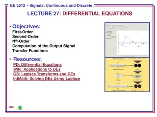
Introduction to Laplace Transforms and Inverse Transformations
In this lecture series, delve into Laplace transforms, their applications in solving differential equations, and the study of inverse Laplace transforms. Explore the concepts with examples, including the Laplace transform of the sine function, roots of denominator polynomials, and the application of the initial and final value theorems. Learn to analyze dynamic systems using lumped-parameter models and Laplace transformations for solving differential equations. Dive into the world of energy absorption, oscillation frequencies, and partial fraction expansions.

Download Presentation

Please find below an Image/Link to download the presentation.
The content on the website is provided AS IS for your information and personal use only. It may not be sold, licensed, or shared on other websites without obtaining consent from the author.If you encounter any issues during the download, it is possible that the publisher has removed the file from their server.
You are allowed to download the files provided on this website for personal or commercial use, subject to the condition that they are used lawfully. All files are the property of their respective owners.
The content on the website is provided AS IS for your information and personal use only. It may not be sold, licensed, or shared on other websites without obtaining consent from the author.
E N D
Presentation Transcript
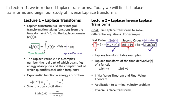
In Lecture 1, we introduced Laplace transforms. Today we will finish Laplace transforms and begin our study of inverse Laplace transforms. Lecture 1 Laplace Transforms Laplace transform is a linear integral transformation taking functions from the time domain (?(?)) to the Laplace domain (?(?)). Lecture 2 Laplace/Inverse Laplace Transforms Goal: Use Laplace transforms to solve differential equations. For example First Order ?[?sin ?? ] Second Order ? ? + ? ? + ?? = ?sin ?? ? ?[? ? ] ? ? + ?? = ?? ?(?) ? ? ? ? ???? = ?(?) ? ? ? = 0 Laplace Domain Time Domain Laplace transform table examples Laplace transform of the time derivative(s) of a function ? ? =? ? ? =? The Laplace variable ? is a complex number, the real part of which quantifies energy absorption and the complex part of which quantifies oscillation frequency. Exponential function energy absorption 1 ? + ? Initial Value Theorem and Final Value Theorem Application to terminal velocity problem Inverse Laplace transforms ? =1 ? ? ??= ? Sine function - oscillation ? ? sin ?? = ?2+ ?2
Example 3: Find the Laplace transform of the sine function ? ? = sin ?? . Step 1: Definition of sine sin ?? =???? ? ??? 2? Step 2: Use linearity of Laplace transform ???? ? ??? 2? =1 ? ???? ? ? ??? ? sin ?? = ? 2? Step 3: Use Laplace transform of exponential 1 ? ? ??= ? + ? 1 ? ????= ? ? ?? ?= ? ?? 1 ? + ?? =1 1 1 ? ? ???= ? ? ?? ?= ? sin ?? ? ?? 2? ? + ?? Step 4: Combine terms by multiplying by complex conjugates ? ? sin ?? = =1 ? + ?? ? ?? ?2+ ?2 ? sin ?? 2? ? ?? ? + ?? ? + ?? ? ?? =1 ? + ?? ? + ?? ?2+ ??? ??? ??2 =1 2?? ? ? sin ?? = ?2+ ?2 ?2+ ?2 2? 2?
Example 3: Find the Laplace transform of the sine function ? ? = sin ?? . Roots of Denominator Polynomial? Step 1: Definition of sine sin ?? =???? ? ??? ?2+ ?2= 0 2? ?2= ?2 Step 2: Use linearity of Laplace transform ???? ? ??? 2? =1 ? = ?? ? ???? ? ? ??? ? sin ?? = ? 2? Roots are imaginary Step 3: Use Laplace transform of exponential Imaginary part of Roots of Denominator Polynomial Energy Conservation/Oscillation 1 ? ? ??= ? + ? 1 ? ????= ? ? ?? ?= ? ?? 1 ? + ?? =1 1 1 ? ? ???= ? ? ?? ?= ? sin ?? ? ?? 2? ? + ?? Step 4: Combine terms by multiplying by complex conjugates ? ? sin ?? = =1 ? + ?? ? ?? ?2+ ?2 ? sin ?? 2? ? ?? ? + ?? ? + ?? ? ?? =1 ? + ?? ? + ?? ?2+ ??? ??? ??2 =1 2?? ? ? sin ?? = ?2+ ?2 ?2+ ?2 2? 2?
The procedure for analyzing dynamic systems is to make a lumped- parameter model of a real system, develop differential equations of motion for the model, and solve using Laplace/Inverse Laplace transforms. ? ? + ? ? + ?? = ?(?) Partial Fraction Expansion
The Laplace transforms of many common functions are known and summarized in tables. Example 1 Find the Laplace transform of ? ? =2 3? 6?. 3? 6?=2 = 3? + 18 ? =1 6 2 3? ? 6? 2 ? ? = ? ? ? ? ? =2 = ? 1 3 ? + 6
The Laplace transforms of many common functions are known and summarized in tables. Example 2 Find the Laplace transform of ? ? = 6cos(8?). ? ? = ? ? ? = ? 6cos(8?) = 6? cos(8?) ? ?2+ 82= 6? ? ? = 6 ?2+ 64
The Laplace transforms of many common functions are known and summarized in tables. Example 3 Find the Laplace transform of ? ? = 4? 6?cos(8?). = ? 4? 6?cos(8?) = 4? ? 6?cos(8?) ? ? = ? ? ? ? =1 6 ?+6 4?+24 Z ? = 4 ?+62+82= ?2+12?+36+64 4?+24 ?2+12?+100 Z(?) =
Example 4: Show that the following is true using the definition of the Laplace transform and integration by parts integration by parts. ?? ?? ? ? = ? = ?? ? ?(0) Step 1: Apply the definition of the Laplace transform Step 4: Apply integration by parts ? ???? ?? ?? ?? ?? ?? ? ???? ? ? = ?? ? ? = ? = 0 0 Step 2: Recall integration by parts = ? ???(?)0 ?(?)( ?? ??)?? ? ? ??? ???? = ??? ???? 0 ? ??? = ?? ??? ?? ? ? ? + ? ? ? = ? ???(?)0 ? ?? ?(?)? ???? Step 3: Make definitions 0 ?? ?? ? ???? ? ???? = ? ? = ?? ?? ) ? ? = ?? ? ?(0 0 0 ?? ??=?? Can also show ?2 ??2 ? ? = ? ?? Initial Conditions ?? ?? ??= ?? ?? ?(?) = ?(?) ? ? = ?2? ? s?(0 ?(0) )
? ? = ?2? ? s?(0 ?(0) ) Let define ? = ?, then we have ? = ? ? ? = ?? ? ?(0) Recall V s = ?[ ?], then we can have ? ? = ? ? = ? ? ? ? 0 ?2? ? s?(0 ?(0) ) ? ?? ? ?(0) ? 0 =
You can go up and down the Laplace transform table knowing that ? is the time derivative and 1/? is the integral.
The Initial Value Theorem and the Final Value Theorem are used to analyze time domain behavior without inverting the Laplace transform. Initial Value Theorem: If the function ?(?) is bounded and lim then the following is true. lim ? 0? ? = lim This provides information about the starting point of a time domain function ?(?) from its Laplace representation ? ? . ? 0? ? exists, ? ??(?) Final Value Theorem: If the function ?(?) is bounded and lim ? 0? ? exists, then the following is true. lim ? ? ? = lim ? 0??(?) This provides information about the ending point of a time domain function ?(?) from its Laplace representation ? ? .
Lets look again at the terminal velocity problem and use what we have learned. Resistance Force Proportional to Velocity ? ??= ?? Newton s Second Law ?, ? ?? ? = ? ? ?? ?(?) ?? ?(?) ??= ? ? ? 0 = 0 ? ? + ?? = ?? ?(?) Initial Value Theorem ? 0 = lim ? 0? ? = lim Apply Laplace Transform ? ??(?) = lim ? ??(?) ?? ?? + ?? ? + ?? ? = ?? ? ? ? ?? = lim ? ? = lim ? = 0 ) ?(?? + ? + ?? ? =?? ? ?? ? ? 0 ? Final Value Theorem ?? ? ? = ???= lim ? ? ? = lim ?? ?(?? + ? ? 0??(?) =?? ) ?(?? + ? = lim ? 0 ? Inverse Laplace transform ) ? ? ? =?
The Laplace transform is applied to linear ODEs, the solution is obtained algebraically in the Laplace domain and then the time domain solution is obtained with the inverse Laplace transform. First Order Linear ODEs Lead to Laplace Functions of the Following Form Use Entry 6 ?0 =?0 1 ? ? = ?1? + ?0 ?1 ? + ?0/?1 Second Order Linear ODEs Lead to Laplace Functions of the Following Form ?1? + ?0 ?2?2+ ?1? + ?0 =?(?) ?(?) ? ? = The Rootsof the denominator polynomial ? ? = ?2?2+ ?1? + ?0 determine the most efficient method to invert the Laplace transform and the form of the solution (oscillatory or exponential).
4 Example 5: Find the inverse Laplace transform of ? ? = 5?+15. Step 1: Factor out the 4 in the numerator and the 5 in the denominator. 5? + 15=4 4 1 ? ? = 5 ? + 3 Step 2: Use linearity of the inverse Laplace transform. ? ? =4 1 5 ? + 3 ? ? = ? 14 1 =4 1 5? 1 5 ? + 3 ? + 3 Step 3: Use table entry 6 in the Laplace transform table. ? ? =4 5? 3? 5? 15=4 4 1 Comment: Suppose ? ? = ? 3. The solution is UNBOUNDED. 5 ? ? =4 5?+3?
For second order denominator polynomials ?(?), the roots of the denominator polynomial determine the form of the inverse transform. Second Order Problem ?1? + ?2 ?1?2+ ?2? +?3 The denominator polynomial is ? ? = ?1?2+ ?2? +?3. There are three possibilities. Real Distinct Roots ?1,2= ?, ?. Partial fractions expansion and entry 6. ?1?+?2 ?1?2+?2?+?3= ?1 (?+?)(?+?) Real Repeated Roots ?1,2= ?, ?. Partial fractions expansion and entries 6 and 7. ? ? = ?1 ?+?2/?1 ?1 ?+?+ ?2 ?+? ? ? = = ?1?+?2 ?1?2+?2?+?3= ?1 ?1 ?+?2/?1 (?+?)2 ?1 ?+?+ ?2 ? ? = = ?+?2 Complex Roots ?1,2= ? ??. Complete the square and use entries 20 and 21. ?1?+?2 ?1?2+?2?+?3= ?1 ?1 ?+?2/?1 (?+?)2+?2 ? ? =
Example 6: The following problem is from RealizIT. Step 1: Factor out the 12 in the numerator and the 18 in the denominator. ? +1 18?2+ 324? + 1170=2 12? + 3 4 ? ? = ?2+ 18? + 65 3 Step 2: Find the roots of the denominator. ?2+ 18? + 65 = 0 182 4(1)(65) 2(1) ?1,2= 18 = 18 324 260 2(1) ?1,2= 18 64 = 18 8 2(1) = 5, 13 2(1) Step 3: Factor and complete a partial fractions expansion. ? + 1/4 ?2+ 18? + 65= ? + 1/4 ?1 ?2 (? + 5)(? + 13)= ? + 5+ ? + 13 Step 4: Find ?1 and ?2 by multiplying through by the denominator and strategically choosing values for s. lim ? 5? + 1/4 = ?1(? + 13) + ?2(? + 5) 19 ? 13? + 1/4 = ?1(? + 13) + ?2(? + 5) 51 4= ?1(8) ?1= 19 32 ? + 1/4 = ?1(? + 13) + ?2(? + 5) 4= ?2( 8) ?2=51 lim 32 Note that since ? is a variable, the values of ?1 and ?2 must be consistent with any values of ?. Thus we can choose ? to aid in finding ?1 and ?2.
Example 6: The following problem is from RealizIT. Step 5: Put in ?1 and ?2. ? ? =2 3 ?2+ 18? + 65 ? + 1/4 ?(?) =2 19 32 1 +51 32 1 3 ? + 5 ? + 13 ?(?) = 19 1 +51 48 1 48 ? + 5 ? + 13 Step 6: Apply table entry 6 to both terms and simplify 51/48 to 17/16. ?(?) = 19 1 +17 16 1 48 ? + 5 ? + 13 ?(?) = 19 48? 5?+17 16? 13? Enter the answers in fractional form. We have worked to be sure that these all come out with even numbers and relatively simple fractions. Real roots of ? ? lead to and exponential, non-oscillatory time domain function.
Example 7: The following problem is from RealizIT. Step 1: Factor out the 7 in the numerator and the 9 in the denominator. 9?2+ 18? + 909=7 7? + 7 ? + 1 ? ? = ?2+ 2? + 101 9 Step 2: Find the roots of the denominator. ?2+ 2? + 101 = 0 22 4(1)(101) 2(1) = 2 20? ?1,2= 2 = 2 4 404 2(1) ?1,2= 2 400 = 1 10? 2(1) 2(1) Step 3: Complete the square in the denominator. ? ? =7 ? + 1 =7 ? + 1 =7 ? + 1 ?2+ 2? + 1 1 + 101 ? + 12+ 100 ? + 12+ 102 9 9 9 Step 4: Use table entry 21. ? ? =7 ? + 1 ? + 12+ 102 9 Complex roots of ? ? lead to a decaying oscillatory time domain function. ? ? =7 9? ?cos 10?
Partial Fraction Expansion When using Laplace to solve LTI ODEs, the solution to the ODE in the Laplace domain is a ratio of polynomials in s. Let ? = ?(?)/? ? where ? ? and ? ? are polynomials in ?. Partial fraction expansion helps to solve for 1 { ( )} q s = L ( ) q t We write 1 m m + + + + ( ) ( ) N s N s N s N N s D s = = 1 n 1 + 0 m s m ( ) q s 1 n + + + D s D s s D 1 )( s 1 0 n z ( ) ( s ) N s s z z = 1 2 ) m s m ( )( ( ) p p p 1 2 n where ?? and ?? are complex numbers.
The main points of Lecture 2 are given. Goal: Use Laplace transforms to solve linear first and second order ordinary differential equations. Laplace transform tables summarize the Laplace transform of many common functions. The properties of Laplace transforms used in conjunction with the tables allow us to find the Laplace transforms of many other functions. For this course, the Laplace transform table it sufficient to all that we do. The Initial Value Theorem (IVT) and Final Value Theorem (FVT) allow us to deduce the behavior of a time domain function ? ? from its Laplace domain representation ?(?). The Laplace transform of the time derivative of a function naturally leads to solutions in the Laplace domain that consist of ratios of polynomials in ?. First order linear ODEs Second order linear ODEs ?1? + ?2 ?1?2+ ?2? +?3 ?0 =?(?) ?(?) ? ? = ? ? = ?1? + ?0 First order systems lead to exponential solutions. Second order systems lead to exponential solutions if the roots of ?(?) are real and distinct and lead to exponentially decaying oscillatory solutions if the roots of ?(?) are complex.
Some notes 1 m m + + + + ( ) ( ) N s N s N s N N s D s = = 1 n 1 + 0 m s m ( ) q s 1 n + + + D s D s s D 1 )( s 1 0 n z ( ) ( s ) N s s z z = 1 2 ) m s m ( )( ( ) p p p 1 2 n If ? = ?, then N(s)/?(?) is exactly proper. If ? > ?, then N(s)/?(?) is strictly proper. Roots of N(s) are ?1,?2, ??. They are called zeros. Roots of D(s) are ?1,?2, ??. They are called poles.
Case #1: All roots are separate. ( ) ( ) k N s D s k k = + + + + 1 2 n k 0 s p s p s p 1 2 n ?0= ?? if n=m or ?0= 0 if m<n. ?0, ?1, ??are called residues. How do we solve for the residues? Example 5: What is the partial fraction expansion of ? + 4( + 2) + s = ( ) q s ( 1)( 5) s s
+ 4( + 2) + s k + k + = = + + 1 2 ( ) q s (1) k 0 ( 1)( 5) 1 5 s s s s Find ?0: ?0= 0 because m=1<n=2 Find ?1: Multiply (1) by s + 1 and evaluate at s = 1 + 4( + 2) + k + s + + = + 2 ( 1 )| ( 1)| k s s = = 1 1 1 s s ( 5) 4(1) (4) ( 1)( 5) s s s + = = 0 1 k k 1 1 Find ?2: Multiply by s + 5 and evaluate at s = 5 k s + + 4( + 2 + ) k + s + + + = + 1 2 ( 5)| ( 5)| ( 5)| s s s = = = 5 5 5 s s s ( 1) ( 5) ( 1)( 5) s s s 4( 3) ( 4) + = = 0 3 k k 2 2 1 + 3 + 1 5 t t = + = = + ( ) ( ) { ( )} 3 q s q t L q s e e 1 5 s s
What if some roots are complex? Example 6: What is s the partial fraction expansion of + + + + + 3( + 1)( + 2)( )( j s 3) 2 s s s = ( ) q s ( 4)( 2 ) s s j Solution + + + + + 3( + 1)( + 2)( )( j s 3) 2 k s s s k + k = + + + 3 1 2 (1) k 0 + + + ( 4)( 2 ) 4 2 2 s s j s s j s j Find ?0: ?0= ??because n=m=3 Find ?1: Multiply by s + 4 and evaluate at s = 4 + + + 3( ( s 1)( 2 2)( + + 3) j 18 5 s + s s = = | k = 1 4 s )( j s 2 )
+ + + + + 3( + 1)( + 2)( )( j s 3) 2 LastSlide k s s s k + k = + + + 3 1 2 k 0 + + + ( 4)( 2 ) 4 2 2 s s j s s j s j Find ?2 Multiply (1) by ? + 2 ? and evaluate at ? = 2 + ? + + + 3( 1)( 4)( + 2)( 2 + + 3) ) 6 5 3 5 s s s = = + | k j = + 2 2 s j ( s s j Find ?3 Multiply (1) by ? + 2 + ? and evaluate at ? = 2 ? + + + 3( 1)( 4)( + 2)( 2 + 3) ) 6 5 3 5 s s s = = | k j = 3 2 s j ( s s j Therefore, + 18/5 s + 6/5 s + + 3/5 j s s 6/5 s j j 3/5 j j j = + + ( ) q s 3 + + + 4 2 2 + + + + + + 18/5 s + 6/5 s + 3/5 j 2 2 6/5 s 3/5 j 2 2 j j s s j j = + + 3 + + 4 2 2 3.6 s + 2.4 6 2) = + Simplification 3 2 + 4 ( 1 s
To find ?1{ ?(?)} note that ?(?) ?(?) + + + ( s ) A s a B at at + = L { cos sin } Ae t Be t 2 2 + ( ) a ?(?) 1 1 ? 1 ?(?) Then, ? ?? 3.6 + 2.4 + + + + 6 1 s ? + ? ? ?2+ ?2 1 ?2+ ?2 1 ?2 ?! ??+1 1 1 1 1 = = + + ( ) L { ( )} L {3} L { } L { } q t q s 2 2 4 s ( 2) 2) 1.2(1) 2) 1 + s s sin?? 2.4( 4 1 t = 3 ( ) 3.6 t + L { } e 2 2 ( s cos?? 4 2 2 t t t = 3 ( ) 3.6 t 2.4 cos 1.2 sin e e t e t ? ??
Case #2- ?(?) has repeated roots ( )( ) ( ) ) ( ) ( ) N s z s z s s z p N s D s = 1 s 2 m m q ( ) ( ) ( s p p 1 2 1 2 q where ?1+ ?2+ + ??. The partial fraction expansion is given by ( ) ( ) ( ) D s s p k + k N s k k p k = + + + + + 1 2 1 k 0 1 ( ) s p ( ) s 1 1 1 1 1 k + 1 n n q q + + + n ( ) s p q q ( ) ( ) 1 s p s p q q q Example7: What is the partial fraction expansion of 1 = ( ) q s 2 + + ( 2)( 1) s s
1 k + k + k + = + + + 3 1 2 1) (1) k 0 2 2 + + 2 1 s s ( 2)( 1) ( s s s Find ?0:?0= 0 because ? = 3 > ? = 2. Find ?1: Multiply (1) by ? + 2 and evaluate at ? = 2. 1 + = = | 1 k = 1 2 s 2 ( 1) s Find ?2: Multiply (1) by (? + 1)2. 2 + + 1 + ( s 1) 2 k s = + + + 1 ( 1) (2) k k s 2 3 2 s Evaluate (2) at ? = 1. 1 + = = | 1 k = 2 1 s 2 s
2 + + LastSlide 1 + ( s 1) 2 k s = + + + 1 ( 1) (2) k k s 2 3 2 s Find ?3: Differentiate (2) with respect to ?. 2 + + + + 1 2) 2( 1) 2 ( ( 1) 2) s s s = + k k 1 3 2 2 + s ( s Evaluate at ? = 1 + 1 2) = = | 1 k = 3 1 s 2 ( s Therefore, + 1 + 1 + 1 = + + ( ) q s 2 2 1 s s ( 1) s
To find ?1{ ?(?)} note that ?(?) ?(?) 1 f s at at = = + = { } { ( )} f t ( ) L te L e a ?(?) 1 1 ? 1 2 + ( ) s a ?(?) Thus, ? ?? + ? + ? ? ?2+ ?2 1 ?2+ ?2 1 ?2 ?! ??+1 1 + 1 + 1 1 1 1 = + + ( ) { } { } { } q t L L L 2 2 1 s + s ( 1) s sin?? 2 t t t = e te e cos?? ? ??


")


, the roots of")


} note that")
 has repeated roots")


} note that")