Optimizing Multiple Regression Models for Fitness Measurements
Explore the application of stepwise regression for predicting oxygen intake based on various exercise test variables in a fitness study dataset from N.C. State University. Learn about model selection criteria, correlation analysis, and scatterplot visualization for effective model building.

Uploaded on | 1 Views
Download Presentation

Please find below an Image/Link to download the presentation.
The content on the website is provided AS IS for your information and personal use only. It may not be sold, licensed, or shared on other websites without obtaining consent from the author. If you encounter any issues during the download, it is possible that the publisher has removed the file from their server.
You are allowed to download the files provided on this website for personal or commercial use, subject to the condition that they are used lawfully. All files are the property of their respective owners.
The content on the website is provided AS IS for your information and personal use only. It may not be sold, licensed, or shared on other websites without obtaining consent from the author.
E N D
Presentation Transcript
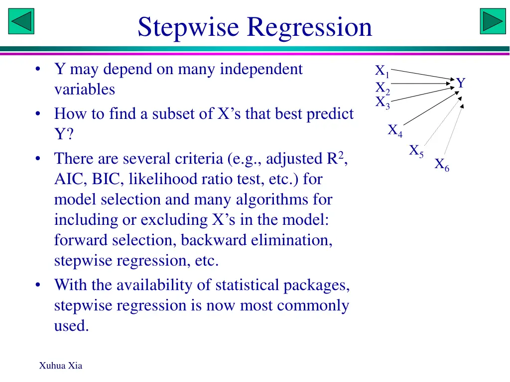
Stepwise Regression Y may depend on many independent variables How to find a subset of X s that best predict Y? There are several criteria (e.g., adjusted R2, AIC, BIC, likelihood ratio test, etc.) for model selection and many algorithms for including or excluding X s in the model: forward selection, backward elimination, stepwise regression, etc. With the availability of statistical packages, stepwise regression is now most commonly used. X1 Y X2 X3 X4 X5 X6 Xuhua Xia
A Data Set for Multiple Regression Measurements on men involved in a physical fitness course at N. C. State University. Fitness is typically measured by oxygen intake rate (oxy) which is difficult (at least cumbersome when one is exercising oneself) to measure. The study goal is to develop an equation to predict oxy based on exercise tests rather than on oxygen consumption measurements. The dataset has 31 observations. The variables in the data set are: age (in years) weight (in kg) oxy (oxygen intake rate, ml per kg body weight per minute) runtime (time to run 1.5 miles, in minutes) rstpulse (heart rate while resting) runpulse (heart rate while running, at the same time when oxygen rate was measured) maxpulse (maximum heart rate recorded while running). Xuhua Xia
oxy age 44 42 40 38 45 49 48 54 51 57 52 40 38 43 44 47 51 49 52 54 49 44 47 44 45 54 51 57 50 51 48 weight 89.47 68.15 75.98 81.87 66.45 81.42 91.63 79.38 67.25 59.08 82.78 75.07 89.02 81.19 73.03 79.15 69.63 73.37 76.32 91.63 76.32 85.84 77.45 81.42 87.66 83.12 77.91 73.37 70.87 73.71 61.24 runtime 11.37 8.17 11.95 8.63 11.12 8.95 10.25 11.17 11.08 9.93 10.5 10.07 9.22 10.85 10.13 10.6 10.95 10.08 9.63 12.88 rstpulse runpulse maxpulse 44.609 59.571 45.681 60.055 44.754 49.156 46.774 46.08 45.118 50.545 47.467 45.313 49.874 49.091 50.541 47.273 40.836 50.388 45.441 39.203 48.673 54.297 44.811 39.442 37.388 51.855 46.672 39.407 54.625 45.79 47.92 62 40 70 48 51 44 48 62 48 49 53 62 55 64 45 47 57 67 48 44 56 45 58 63 56 50 48 58 48 59 52 178 166 176 170 176 180 162 156 172 148 170 185 178 162 168 162 168 168 164 168 186 156 176 174 186 166 162 174 146 186 170 182 172 180 186 176 185 164 165 172 155 172 185 180 170 168 164 172 168 166 172 188 168 176 176 192 170 168 176 155 188 176 9.4 8.65 11.63 13.08 14.03 10.33 10 12.63 8.92 10.47 11.5 Xuhua Xia
Correlation matrix age weight oxy runtime rstpulse runpulse maxpulse age 1.00000 -0.23354 -0.30459 0.18875 -0.16410 -0.33787 -0.43292 0.2061 0.0957 0.3092 0.3777 0.0630 0.0150 weight -0.23354 1.00000 -0.16275 0.14351 0.04397 0.18152 0.24938 0.2061 0.3817 0.4412 0.8143 0.3284 0.1761 oxy -0.30459 -0.16275 1.00000 -0.86219 -0.39936 -0.39797 -0.23674 0.0957 0.3817 <.0001 0.0260 0.0266 0.1997 runtime 0.18875 0.14351 -0.86219 1.00000 0.45038 0.31365 0.22610 0.3092 0.4412 <.0001 0.0110 0.0858 0.2213 rstpulse -0.16410 0.04397 -0.39936 0.45038 1.00000 0.35246 0.30512 0.3777 0.8143 0.0260 0.0110 0.0518 0.0951 runpulse -0.33787 0.18152 -0.39797 0.31365 0.35246 1.00000 0.92975 0.0630 0.3284 0.0266 0.0858 0.0518 <.0001 maxpulse -0.43292 0.24938 -0.23674 0.22610 0.30512 0.92975 1.00000 0.0150 0.1761 0.1997 0.2213 0.0951 <.0001 Xuhua Xia
Scatterplot matrix Xuhua Xia
rcorr in Hmisc oxy age weight runtime rstpulse runpulse maxpulse oxy 1.00 -0.30 -0.16 -0.86 -0.40 -0.40 -0.24 age -0.30 1.00 -0.23 0.19 -0.16 -0.34 -0.43 weight -0.16 -0.23 1.00 0.14 0.04 0.18 0.25 runtime -0.86 0.19 0.14 1.00 0.45 0.31 0.23 rstpulse -0.40 -0.16 0.04 0.45 1.00 0.35 0.31 runpulse -0.40 -0.34 0.18 0.31 0.35 1.00 0.93 maxpulse -0.24 -0.43 0.25 0.23 0.31 0.93 1.00 P oxy age weight runtime rstpulse runpulse maxpulse oxy 0.0957 0.3817 0.0000 0.0260 0.0266 0.1997 age 0.0957 0.2061 0.3092 0.3777 0.0630 0.0150 weight 0.3817 0.2061 0.4412 0.8143 0.3284 0.1761 runtime 0.0000 0.3092 0.4412 0.0110 0.0858 0.2213 rstpulse 0.0260 0.3777 0.8143 0.0110 0.0518 0.0951 runpulse 0.0266 0.0630 0.3284 0.0858 0.0518 0.0000 maxpulse 0.1997 0.0150 0.1761 0.2213 0.0951 0.0000 > print(rmat) oxy age weight runtime rstpulse runpulse maxpulse oxy 1.00 -0.30 -0.16 -0.86 -0.40 -0.40 -0.24 age -0.30 1.00 -0.23 0.19 -0.16 -0.34 -0.43 weight -0.16 -0.23 1.00 0.14 0.04 0.18 0.25 runtime -0.86 0.19 0.14 1.00 0.45 0.31 0.23 rstpulse -0.40 -0.16 0.04 0.45 1.00 0.35 0.31 runpulse -0.40 -0.34 0.18 0.31 0.35 1.00 0.93 maxpulse -0.24 -0.43 0.25 0.23 0.31 0.93 1.00
Backward elimination Start: AIC=58.16 oxy ~ age + weight + runtime + rstpulse + runpulse + maxpulse the current model, i.e., without eliminating rstpulse Df Sum of Sq RSS AIC - rstpulse 1 0.571 129.41 56.299 <none> 128.84 58.162 - weight 1 9.911 138.75 58.459 - maxpulse 1 26.491 155.33 61.958 - age 1 27.746 156.58 62.208 - runpulse 1 51.058 179.90 66.510 - runtime 1 250.822 379.66 89.664 + 2( 1) p = + ( ) ln( ( )) AIC p SSE p n + ( 1)ln( ) n p n = + ( ) ln( ( )) BIC p SSE p Step: AIC=56.3 oxy ~ age + weight + runtime + runpulse + maxpulse Df Sum of Sq RSS AIC <none> 129.41 56.299 - weight 1 9.52 138.93 56.499 - maxpulse 1 26.83 156.23 60.139 - age 1 27.37 156.78 60.247 - runpulse 1 52.60 182.00 64.871 - runtime 1 320.36 449.77 92.917 Xuhua Xia
Forward addition Start: AIC=104.7 oxy ~ 1 Step: AIC=63.9 oxy ~ runtime + age IVs whose addition will improve fit Df Sum of Sq RSS AIC + runtime 1 632.90 218.48 64.534 + rstpulse 1 135.78 715.60 101.313 + runpulse 1 134.84 716.54 101.354 + age 1 78.99 772.39 103.681 <none> 851.38 104.699 + maxpulse 1 47.72 803.67 104.911 + weight 1 22.55 828.83 105.867 Df Sum of Sq RSS AIC + runpulse 1 39.885 160.83 59.037 + maxpulse 1 14.885 185.83 63.516 <none> 200.72 63.905 + weight 1 5.605 195.11 65.027 + rstpulse 1 2.641 198.07 65.494 Step: AIC=59.04 oxy ~ runtime + age + runpulse IVs whose addition will make it worse Step: AIC=64.53 oxy ~ runtime Df Sum of Sq RSS AIC + maxpulse 1 21.9007 138.93 56.499 <none> 160.83 59.037 + weight 1 4.5958 156.24 60.139 + rstpulse 1 0.4901 160.34 60.943 Df Sum of Sq RSS AIC + age 1 17.7656 200.72 63.905 + runpulse 1 15.3621 203.12 64.274 <none> 218.48 64.534 + maxpulse 1 1.5674 216.91 66.311 + weight 1 1.3236 217.16 66.346 + rstpulse 1 0.1301 218.35 66.516 Step: AIC=56.5 oxy ~ runtime + age + runpulse + maxpulse Xuhua Xia
R Functions Two R functions for computing Pearson correlation: cor in basic package does not provide associated p, and rcorr in the Hmisc package includes p. library(Hmisc) cor(myD,method="pearson|spearman") pairs(~age+weight+runtime+rstpulse+runpulse+maxpulse+oxy) rmat<-rcorr(as.matrix(myD), type="pearson|spearman") rmat print(rmat[1],digits=5) fit<-lm(oxy~age+weight+runtime+rstpulse+runpulse+maxpulse) anova(fit) summary(fit) full.model<-lm(oxy~age+weight+runtime+rstpulse+runpulse+maxpulse) best.model<-step(full.model,direction="backward") min.model<-lm(oxy~1) best.model<-step(min.model,direction="forward", scope="~age+weight+runtime+rstpulse+runpulse+maxpulse") new<-data.frame(age=50,weight=82,......) predict(fit,new,interval="confidence") predict(fit,new,interval="prediction") Xuhua Xia
Package leaps Package leaps includes a function leaps that offers two more criteria for model selection: 1) adjusted r2 2) Mallow's Cp (which is used less frequently now) The input to leaps is not a data frame but a vector for DV and a matrix for IVs: x<-as.matrix(myD) DV<-x[,1] IV<-x[,2:7] library(leaps) solR2a<-leaps(IV, DV, names=names(myD)[2:7], method="adjr2") solCp<-leaps(IV, DV, names=names(myD)[2:7], method="Cp") Xuhua Xia
leaps evaluates all linear models $which age weight runtime rstpulse runpulse maxpulse 1 FALSE FALSE TRUE FALSE FALSE FALSE 1 FALSE FALSE FALSE TRUE FALSE FALSE 1 FALSE FALSE FALSE FALSE TRUE FALSE 1 TRUE FALSE FALSE FALSE FALSE FALSE 1 FALSE FALSE FALSE FALSE FALSE TRUE 1 FALSE TRUE FALSE FALSE FALSE FALSE 2 TRUE FALSE TRUE FALSE FALSE FALSE 2 FALSE FALSE TRUE FALSE TRUE FALSE 2 FALSE FALSE TRUE FALSE FALSE TRUE 2 FALSE TRUE TRUE FALSE FALSE FALSE 2 FALSE FALSE TRUE TRUE FALSE FALSE 2 TRUE FALSE FALSE FALSE TRUE FALSE 2 TRUE FALSE FALSE TRUE FALSE FALSE 2 FALSE FALSE FALSE FALSE TRUE TRUE 2 TRUE FALSE FALSE FALSE FALSE TRUE 2 FALSE FALSE FALSE TRUE TRUE FALSE 3 TRUE FALSE TRUE FALSE TRUE FALSE 3 FALSE FALSE TRUE FALSE TRUE TRUE 3 TRUE FALSE TRUE FALSE FALSE TRUE 3 TRUE TRUE TRUE FALSE FALSE FALSE 3 TRUE FALSE TRUE TRUE FALSE FALSE 3 FALSE FALSE TRUE TRUE TRUE FALSE 3 FALSE TRUE TRUE FALSE TRUE FALSE 3 FALSE TRUE TRUE FALSE FALSE TRUE 3 FALSE FALSE TRUE TRUE FALSE TRUE 3 FALSE TRUE TRUE TRUE FALSE FALSE The best model is one with the greatest adjusted r2 or a Cp closest to the total number of IVs (6 in our case) The next two slides show results of evaluation Xuhua Xia
Model evaluation: adjusted r2 The number of coefficients in each model $size [1] 2 2 2 2 2 2 3 3 3 3 3 3 3 3 3 3 4 4 4 4 4 4 4 4 4 4 5 5 5 5 5 5 5 5 5 5 6 6 [39] 6 6 6 6 7 $adjr2 [1] 0.734531140 0.130502041 0.129362176 0.061492963 0.023495780 [6] -0.007080873 0.747407426 0.744382656 0.727022568 0.726715841 [11] 0.725213882 0.331423675 0.250289567 0.238663728 0.207123289 [16] 0.180390053 0.790104958 0.788876048 0.757477967 0.745367336 [21] 0.741499364 0.735442756 0.735365598 0.717949838 0.716918697 [26] 0.716790424 0.811713247 0.788260638 0.787518105 0.782696332 [31] 0.781231246 0.753335728 0.750114011 0.740422515 0.725675821 [36] 0.707129090 0.817602176 0.804437584 0.781067331 0.779299361 [41] 0.746441303 0.464879114 0.810839895 Given the set of adjusted r2 values for the 43 alternative models, which one is the maximum? Find the max adjusted r2 Find the index of the max adjusted r2 Show the best model maxAdjR2<-max(solR2a$adjr2); bestModelInd<-match(maxAdjR2,solR2a$adjr2) solR2a$which[bestModelInd,] Find the index of the max adjusted r2 bestModelInd<-which.max(solR2a$adjr2) Xuhua Xia
leaps output for Cp: 2 The number of coefficients in each model $size [1] 2 2 2 2 2 2 3 3 3 3 3 3 3 3 3 3 4 4 4 4 4 4 4 4 4 4 5 5 5 5 5 5 5 5 5 5 6 6 [39] 6 6 6 6 7 $Cp [1] 13.698840 106.302108 106.476860 116.881841 122.707162 127.394846 [7] 12.389449 12.837184 15.406872 15.452274 15.674598 73.964510 [13] 85.974204 87.695093 92.363796 96.320923 6.959627 7.135037 [19] 11.616680 13.345306 13.897406 14.761903 14.772916 17.258776 [25] 17.405958 17.424267 4.879958 8.103512 8.205573 8.868324 [31] 9.069700 12.903931 13.346755 14.678848 16.705777 19.255019 [37] 5.106275 6.846150 9.934837 10.168497 14.511122 51.723275 [43] 7.000000 Given the set of Cp values for the 43 alternative models, which one is closest to 6? solCp bestModelInd<-which(abs(solCp$Cp-6)==min(abs(solCp$Cp-6))) solCp$which[bestModelInd,] This leads to a model that is suboptimal based on AIC or adjusted r2
Criteria used in model selection 1 n Ra2 Cp SBC (BIC) AIC Significance level 2 2 = 1 1 ( 1 ) Ra R n m Burnham, K. P. and D. R. Anderson. 2002 Model selection and multimodel inference: a practical information-theoretic approach. 2nd ed. Springer. (Best book on model selection) Xuhua Xia