Synchronous Machine Modeling in Power Systems
Electric machines play a crucial role in converting energy between mechanical and electrical forms. This lecture delves into synchronous machine modeling, explaining the fundamental concepts such as d-q reference frames, transformations, and the key laws governing their operation. Through detailed explanations and illustrations, the complexities of synchronous generators and motors are unraveled, shedding light on their essential role in power systems.

Download Presentation

Please find below an Image/Link to download the presentation.
The content on the website is provided AS IS for your information and personal use only. It may not be sold, licensed, or shared on other websites without obtaining consent from the author.If you encounter any issues during the download, it is possible that the publisher has removed the file from their server.
You are allowed to download the files provided on this website for personal or commercial use, subject to the condition that they are used lawfully. All files are the property of their respective owners.
The content on the website is provided AS IS for your information and personal use only. It may not be sold, licensed, or shared on other websites without obtaining consent from the author.
E N D
Presentation Transcript
ECE 576 Power System Dynamics and Stability Lecture 6: Synchronous Machine Modeling Prof. Tom Overbye Dept. of Electrical and Computer Engineering University of Illinois at Urbana-Champaign overbye@illinois.edu Special Guest: TA Soobae Kim 1
Announcements Read Chapter 3 2
Synchronous Machine Modeling Electric machines are used to convert mechanical energy into electrical energy (generators) and from electrical energy into mechanical energy (motors) Many devices can operate in either mode, but are usually customized for one or the other Vast majority of electricity is generated using synchronous generators and some is consumed using synchronous motors, so that is where we'll start Much literature on subject, and sometimes overly confusing with the use of different conventions and nominclature 3
Synchronous Machine Modeling 3 bal. windings (a,b,c) stator Field winding (fd) on rotor Damper in d axis (1d) on rotor 2 dampers in q axis (1q, 2q) on rotor 4
Dq0 Reference Frame Stator is stationary and rotor is rotating at synchronous speed Rotor values need to be transformed to fixed reference frame for analysis This is done using Park's transformation into what is known as the dq0 reference frame (direct, quadrature, zero) Convention used here is the q-axis leads the d-axis (which is the IEEE standard) Others (such as Anderson and Fouad) use a q-axis lagging convention 5
Fundamental Laws Kirchhoff s Voltage Law, Ohm s Law, Faraday s Law, Newton s Second Law Stator Rotor Shaft d d fd 2 P d = + v fd fd i r a = + shaft dt d P dt = v a s i r fd dt a dt d 2 = 1 d = + d J T T T v i r m e f b = + 1 1 1 d d d v b s i r dt b dt d dt d 1 q = + v 1 1 q q i r 1 q c = + dt d v c s i r c 2 q = + v i r 2 2 2 q q q dt 6
Dq0 transformations v v v v v d a or , dqo T i q b v c o = v v v v v a d 1 dqo T b q v c o 7
Dq0 transformations 2 2 P P P shaft shaft shaft + sin sin sin 2 P 2 P 3 2 3 2 P 3 2 3 2 3 shaft shaft shaft + cos cos cos dqo T 2 2 2 1 2 1 2 1 2 with the inverse, sin P P cos 1 shaft shaft 2 2 2 2 P P dqo T 1 = sin cos 1 shaft shaft 2 P 3 2 P 3 2 2 + + sin cos 1 shaft shaft 2 3 2 3 8
Dq0 transformations Note: This transformation is not power invariant. This means that some unusual things will happen when we use it. Example: If the magnetic circuit is assumed to be linear abc = Li abc (symmetric) T 1 = TLT dqo i 1 abc dqo = TLT dqo i Not symmetric if T is not power invariant. 9
Transformed System Stator Rotor Shaft d d 2 P fd = + v fd fd r i d shaft dt d = fd d = + v s d r i dt d q dt d dt d 2 P dt 1 d = + v 1 1 d d r i = J T T T 1 d q = + + m e f dt v s q r i q d d 1 q = + v 1 1 q q r i d 1 q o = + v s o r i dt d o dt 2 q = + v r i 2 2 2 q q q dt 10
Electrical & Mechanical Relationships Electrical system: d dt = + (voltage) v iR d 2 = + (power) vi i R idt Mechanical system: 2 P d dt = (torque) J T T T m e f 2 2 P 2 P 2 P 2 P d dt = (power) J T T T m e f 11
Derive Torque Torque is derived by looking at the overall energy balance in the system Three systems: electrical, mechanical and the coupling magnetic field Electrical system losses in form of resistance Mechanical system losses in the form of friction Coupling field is assumed to be lossless, hence we can track how energy moves between the electrical and mechanical systems 12
Energy Conversion Look at the instantaneous power: 3 3 + + = + + 3 v i v i v i v i v i v i a a b b c c d d q q o o 2 2 13
Change to Conservation of Power = + + + + + P v i v i v i v i v i v i 1 1 1 1 in a a b b c c fd fd d d q q elect + v i 2 2 q 2 q ( ) 2 2 2 2 1 2 1 2 2 = + + + + + + P r i i i r i r i r i r i 1 1 2 lost s a b c fd fd d d q q q q elect d d d d d fd 1 a b c d = + + + + P i i i i i 1 trans a b c fd d dt dt dt dt dt elect d d 1 2 q q + + i i 1 2 q q dt dt 14
With the Transformed Variables 3 3 = + + + + 3 P v i v i v i v i v 1 i 1 in d d q q o o fd fd d d 2 2 elect + + v 1 i v i 1 2 2 q q q q 3 3 2 d i 2 q i 2 o i 2 fd 2 1 i = + + + + 3 lost P r r r r i 1 r s s s fd d d 2 2 elect 2 1 i 2 2 i + + 1 r r 2 q q q q 15
With the Transformed Variables shaft shaft d d 3 3 3 P 2 d P 2 d = + + P i i i trans q d d d q 2 2 2 dt dt dt elect d d 3 d d q fd 1 o d + + + + 3 i i i i 1 q o fd d 2 dt dt dt dt d d 1 2 q q + + i i 1 2 q q dt dt 16
Change in Coupling Field Energy dW dt d da db 2 f = + + Te ai bi P dt dt dt dfd dc d 1 d + + +ci i1 i d fd dt dt dt d d 1 2 q q + i1 i2 + q q dt dt This requires the lossless coupling field assumption 17
Change in Coupling Field Energy For independent states , a, b, c, fd, 1d, 1q, 2q dW dt W W W d da db f f f f = + + dt dt dt a b dfd W W W dc d f f f 1 d + + + dt dt dt 1 c d fd W W d d 1 2 q q f f + + dt dt 1 2 q q 18
Equate the Coefficients W W 2 P f f = = T i etc. e a a There are eight such reciprocity conditions for this model. These are key conditions i.e. the first one gives an expression for the torque in terms of the coupling field energy. 19
Equate the Coefficients 3 2 2 P W ( ) f + d q i q d i T = e shaft W W W 3 2 3 f f f = = = , , 3 i i i d q o 2 d q o W W W W f f f f = = = = , , , i i i i fd 1 1 2 d q q fd 1 1 2 d q q These are key conditions i.e. the first one gives an expression for the torque in terms of the coupling field energy. 20
Coupling Field Energy The coupling field energy is calculated using a path independent integration For integral to be path independent, the partial derivatives of all integrands with respect to the other states must be equal 3 For example, 2 fd d i i fd = d Since integration is path independent, choose a convenient path Start with a de-energized system so all variables are zero Integrate shaft position while other variables are zero, hence no energy Integrate sources in sequence with shaft at final shaft value 21
Do the Integration ) ( shaft 3 2 2 P o f = + W W i i d f d q q d shaft o shaft q d o 3 2 3 2 + + + 3 i d d i d q i d o d q o o d o q o o 1 2 fd q q 1 d 1 1 + + + + i d i d i d q i d 1 1 2 2 fd fd d d q q q o fd o d o q o 1 1 2 q 22
Torque Assume: iq, id, io, ifd, i1d, i1q, i2q are independent of shaft (current/flux linkage relationship is independent of shaft) Then Wf will be independent of shaft as well Since we have ( d q q d shaft 2 2 W 3 P ) f = + = i i T 0 e ( ) 3 P 2 = T i i e d q q d 2 23
Define Unscaled Variables P d fd shaft = + t fd fd r i v s fd dt 2 d 1 d = + 1 1 d d r i v s is the rated synchronous speed d plays an important role! 1 d dt d 1 q = + 1 1 q q r i v 1 q dt d d = + + s d r i v d q d 2 q dt d dt d dt = + r i v 2 2 2 q q q dt q = + s q r i v d q d dt d = s o = + s o r i v 2 p dt 3 2 P ( ) o = + J T d q i q d i T m f 2 24
Convert to Per Unit As with power flow, values are usually expressed in per unit, here on the machine power rating P I V = Base Base Base Two common sign conventions for current: motor has positive currents into machine, generator has positive out of the machine Modify the flux linkage current relationship to account for the non power invariant dqo transformation 25
Convert to Per Unit v v v a b c , , , V V V a b c BABC V i I BABC V i I BABC V i I a b c , , I I I a b c BABC BABC BABC a b c , , a b c BABC BABC BABC where VBABCis rated RMS line-to-neutral stator voltage and P I V BABC V B , BABC BABC 3 BABC B 26
Convert to Per Unit v v v q d o , , , V V V d q o BDQ V i I BDQ V i I BDQ V i q d o , , I I I d q o I BDQ BDQ BDQ q d o , , d q o BDQ BDQ BDQ where VBDQ is rated peak line-to-neutral stator voltage and 2 , 3 BDQ V BDQ V P B I BDQ BDQ B 27
Convert to Per Unit v v v v 1 2 fd q q 1 d , , , V V V V 1 1 2 fd d q q BFD V i I B D V i I B Q V i B Q V 1 1 2 i 1 2 fd q q 1 d , , , I I I I 1 1 2 fd d q q I I 1 1 2 BFD B D B Q B Q 1 2 fd q q 1 d , , , 1 1 2 fd d q q 1 1 2 BFD B D B Q B Q Hence the variables are just normalized flux linkages 28
Convert to Per Unit Where the rotor circuit base voltages are P V I P V I And the rotor circuit base flux linkages are V P B B , , B D V 1 BFD I 1 BFD B D P B B , B Q V 1 2 B Q I 1 2 B Q B Q B D V 1 BFD , , 1 BFD B D B B B Q V B Q V 1 2 , 1 2 B Q B Q B B 29
Convert to Per Unit r r r fd 1 s d , , , R R R 1 s fd d Z Z Z 1 BDQ BFD r q Z B D r Z 1 2 q , , R R 1 2 q q 1 2 B Q B Q BDQ V I BFD V I B D V I 1 , , , Z Z Z 1 BDQ BFD B D 1 BDQ BFD V I B D V I 1 2 B Q B Q , Z Z 1 2 B Q B Q 1 2 B Q B Q 30
Convert to Per Unit Almost done with the per unit conversions! Finally define inertia constants and torque 2 1 2 2 P ( ) J 2H B = , H M S B s T T T T T T S fw , , , m e T ELEC T T T B M FW B 2 P B B B B 31
Synchronous Machine Equations 1 d d 1 d = + + fd R I V = + R I V s d q d fd fd fd dt dt s s s d 1 1 d q = + R I V 1 d = + R I V s q d q 1 1 1 dt d d d dt d s s s 1 1 d o = + R I V 1 q = + R I V s o o dt 1 1 1 q q q s dt s d 1 2 q = + 2 R I V 2 2 q q dt d dt s = s 2 H d ( ) = T d q I q d I T M FW dt s 32
Sinusoidal Steady-State ( ) = + 2 cos V V t a s s vs Here we consider the application to balanced, sinusoidal conditions 2 = + 2 cos V V t b s s vs 3 2 = + + 2 cos V V t c s s vs 3 ( ) = + 2 cos I I t a s s is 2 = + 2 cos I I t b s s is 3 2 = + + 2 cos I I t c s s is 3 33
Transforming to dq0 2 V BABC V P s = shaft sin V t d s vs 2 BDQ V 2 V BABC V P s = shaft cos V t q s vs 2 BDQ V = 0 V o 2 s BABC I I I P = shaft sin I t d s is 2 BDQ 2 s BABC I I I P = shaft cos I t q s is 2 BDQ = 0 I o 34
Simplifying Using Recall that P shaft t s 2 The conclusion is if we know , then we can easily relate the phase to the dq values! ( ( ( ( ) ) = sin V V d s vs Hence = cos V V q s vs ) ) = sin I I d s is = cos I I q s is These algebraic equations can be written as complex equations, ) ( ( ( ) j /2 j vs + = V jV e V e s d q ) ( ) j /2 j is + = I jI e I e s d q 35
Summary So Far The model as developed so far has been derived using the following assumptions The stator has three coils in a balanced configuration, spaced 120 electrical degrees apart Rotor has four coils in a balanced configuration located 90 electrical degrees apart Relationship between the flux linkages and currents must reflect a conservative coupling field The relationships between the flux linkages and currents must be independent of shaft when expressed in the dq0 coordinate system 36
Assuming a Linear Magnetic Circuit If the flux linkages are assumed to be a linear function of the currents then we can write i i i The rotor self- inductance matrix Lrr is independent of shaft a a ( ) ( ) shaft shaft L L b b ss sr c c = i i fd fd ( ) ( ) 1 1 i i d d shaft shaft L L rs rr 1 1 q q 2 2 q q 37
Inductive Dependence on Shaft Angle L12 = 0 L12 = + maximum L12 = - maximum 38
Stator Inductances The self inductance for each stator winding has a portion that is due to the leakage flux which does not cross the air gap, Lls The other portion of the self inductance is due to flux crossing the air gap and can be modeled for phase a as + P cos( ) L L A B shaft Mutual inductance between the stator windings is modeled as 1L L P offset 2 The offset angle is either 2 /3 or -2 /3 + cos( ) A B shaft 39
Conversion to dq0 for Angle Independence i i i d d q q 1 dqo sr T L o o dqo ss dqo T L T = i i fd fd 1 1 i i d d 1 L rs dqo L T rr 1 1 q q 2 2 q q 40
Conversion to dq0 for Angle Independence ( 3 2 3 2 ( 3 2 3 2 L i ) 3 3 3 3 = + + + L L i sfd fd L i 1 1 s d d L i ( ) + , L L L d s md d md A B = + + sfd d L i L i L i 1 1 fd d d fd fdfd fd ( ) L L L mq A B = + + s d d L i L ) i 1 1 1 d d d L i 1 1 1 d fd d fd = + + + L L i 1 1 s q q L i s q L i 2 2 q s mq q q = + + s q q L i 1 1 1 q q q L i 1 2 q q L i 1 1 2 q q = + + s q q L i 1 2 1 q q q L i 2 2 q q L i 2 2 2 q q = o s o 41
Convert to Normalized at f = s Convert to per unit, and assume frequency of s Then define new per unit reactance variables , s md BDQ BDQ Z Z L L X X Z Z L L X X Z Z + L L L s mq , s s s md X X X mq Z BDQ L L s fdfd s fd1d sfd , , s 1d1d X fd 1d fd1d Z L BFD B1D BFD L Z s1d L L s 1q1q s 2q2q s 1q2q s1q , , X 1q 2q 1q2q B1Q B2Q X B1Q s2q , X X X X X fd fd md 1d 1d md , X X X X X + X 1q 1q mq , 2q 2 q X mq X X X X X d s md q s mq 42
Normalized Equations ( ) = + + X I X I X I 1 d d d I md X fd I md d ( ( ) ) = + + X c X I 1 fd md d fd fd d + md d = = + X I c X I X I 1 c 1 1 d md d d md fd d d X X 1 1 2 q q X fd d X , c c 1 X d q d ( ) md mq + + I X I X I 1 2 q q q mq q mq q ( ( ) ) = + + X I X I c X I 1 1 1 2 q mq q q q q mq q = + + X I c X I X I 2 c 1 2 2 q mq q q mq q q q 1 q ( ) = X I o s o 43