In the realm of transmission lines, understanding the theory becomes pivotal when the line's length is substantial compared to the wavelength. This theory delves into the intricacies of transmission line behavior and the importance of per-unit-length parameters like capacitance, inductance, resistance, and conductance. The equal and opposite currents on the two conductors play a crucial role in the transmission line's operation. The content also delves into differential equations and time-harmonic waves in the context of transmission lines.
Please find below an Image/Link to download the presentation.
The content on the website is provided AS IS for your information and personal use only. It may not be sold, licensed, or shared on other websites without obtaining consent from the author. If you encounter any issues during the download, it is possible that the publisher has removed the file from their server.
You are allowed to download the files provided on this website for personal or commercial use, subject to the condition that they are used lawfully. All files are the property of their respective owners.
The content on the website is provided AS IS for your information and personal use only. It may not be sold, licensed, or shared on other websites without obtaining consent from the author.
Transmission Line (cont.) ( ) , i z t ( ) + + + + + + + - - - - - - - - - - , v z t x x x B z ( ) R z ( ) + , i z z t L z , i z t + + ( ( ) ) + , v z z t G z C z , v z t - - z There are equal and opposite currents on the two conductors. 4
Transmission Line (cont.) ( ) R z ( ) + , i z z t L z , i z t + + ( ( ) ) + , v z z t G z C z , v z t - - z ( , ) i z t t = + + + ( , ) v z t ( , ) z t ( , ) i z t R z v z L z v z + ( , ) z t = + + , ) z t G z + + ( , ) i z t ( , ) z t ( i z v z C z t 5
TEM Transmission Line (cont.) Hence + ( , ) z t ( , ) v z t ( , ) i z t t v z = ( , ) Ri z t L z + v z + ( , ) z t ( , ) i z t ( , ) z t i z = + ( , ) z t Gv z C z t Now let z 0: v z i z i t = Ri L v t = Gv C 6
TEM Transmission Line (cont.) To combine these, take the derivative of the first one with respect to z: v i z i z i t i z 2 = R L z z 2 = R L t v t v t v 2 = R Gv C L G C t 2 7
TEM Transmission Line (cont.) v v t v t v 2 2 = Gv C R L G C z t 2 2 Hence, we have: v v t v 2 2 ( ) + = ( ) 0 RG v RC LG LC z t 2 2 The same differential equation also holds for i. 8
TEM Transmission Line (cont.) Time-Harmonic (=Sinusoidal) Waves: j = + = ( ) v t cos( ), (phasor of ), A t V Ae v j t v v t v 2 2 ( ) + = ( ) 0 RG v RC LG LC z t 2 2 d V dz 2 ( ) + = ( ) ( ) 0 RG V RC LG j V LC V 2 2 9
TEM Transmission Line (cont.) d V dz 2 ( ) ( ) = + + ( ) RG V j RC LG V LC V 2 2 Note that + + = + j L G + j C ( ) ( )( ) RG j RC LG LC R 2 = = + + Z Y R G j L j C = = series impedance / unit length parallel admittance / unit length d V dz 2 = ( ) ZY V Then we can write: 2 10
Complex Numbers = 1 j = + z x jy = = je z z z ( ) z = Re z x = Im( ) y j = cos sin e j
Complex Numbers Rectangular to Polar Conversion, Programming = + z x jy j = z e 2 2 = + x y x 1 cos (0 ), 0 y = x 1 + cos , 0 y y x 1 tan , 0 x = = undefined, 0, 0 x y = = / 2, 0, 0 x y = / 2, 0, 0 x y y x 1 + tan , 0 x
TEM Transmission Line (cont.) ( ) d V z dz 2 ( ) = ZY V z Then 2 Define 2 2 Solution: + z z = + ( ) V z Ae Be z : voltage wave propagating in + direction Ae z + z : voltage wave propagating in direction Be z is called the propagation constant . 1/2 = + j L G + j C ( )( ) R 16
TEM Transmission Line (cont.) 1/2 = + j L G + j C ( )( ) R We choose the principal square root. re = j Principal square root: z = /2 j z r e ( ) z Re 0 Hence = + j L G + j C ( )( ) R Re 0 17
TEM Transmission Line (cont.) = + j L G + j C ( )( ) R = + j Denote: = propagation constant 1/m = attenuationcontant [np/m] = phaseconstant rad/m = Re 0 18
TEM Transmission Line (cont.) Wave traveling in +z direction: ( ) ( ) j z = = z z = + V z Ae Ae e j Wave is attenuating as it propagates. Wave traveling in z direction: ( ) ( ) = + + + + j z = = j z z V z Ae Ae e Wave is attenuating as it propagates. 19
TEM Transmission Line (cont.) ( ) j z = z Attenuation in dB/m: V z Ae e V V = Attenuation in dB 20log out 10 in z A e = 20log 10 A ( )( ) = = 20 0.4343 8.686 z z ( ) x ( ) x = Note: log 0.4343 ln 10 = (dB/m) Np: neper, 1 Np = 8.686 (Np/m) e = 1 0.37 20
Wavenumber Notation ( ) j z = = z z = + V z Ae Ae e j ( ) j z = = = jk z z zk j V z Ae Ae e z = jk z = + j L G + j C ( )( ) R "(complex) propagationconstant" = + j L G + j C ( )( ) zk j R "(complex) wavenumber" 21
TEM Transmission Line (cont.) Forward travelling wave (a wave traveling in the positive z direction): + + + j z z z = = ( ) z V V e V e e 0 0 ( ( ) + + j z j t z = ( , ) z t Re v V e e e 0 ) ( ) + j z j t j z = Re V e e e e 0 ( ) + z = + cos V e t z The wave repeats when: 0 = 2 g t = 0 g Hence: + z V e 0 2 = z g snapshot of wave 22
Phase Velocity Let s track the velocity of a fixed point on the wave (a point of constant phase), e.g., the crest of the wave. p v (phase velocity) z + + z = + ( , ) z t cos( ) v V e t z 0 23
Characteristic Impedance Z0 ( ) z + I + ( ) z + V z Assumption: A wave is traveling in the positive z direction. + ( ) : characteristic impedance ( ) z V I z Z 0 + + + z = ( ) z V V e + 0 V I 0 + = Z so 0 + + z = ( ) z I I e 0 0 (Note: Z0 is a number, not a function of z.) 25
Characteristic Impedance Z0(cont.) Use first Telegrapher s Equation: v z i t = Ri L so dV dz = j LI = RI ZI + + = = z ( ) z V V e 0 + Recall: + z ( ) z I I e 0 + + V e = z z Hence ZI e 0 0 26
Characteristic Impedance Z0(cont.) + V I Z Z ZY 0 + From this we have: = = = Z 0 0 Use: = = + + Z Y R G j L j C Both are in the first quadrant = ZY first quadrant = / Z Z ZY right -half plane 0 Re 0 Z 0 Z Y = (principal square root) Z 0 27
RLGC from Z0 and + + 1 Z Y R G j L j C = = Z 0 Y 0 = + j L G + j C ( )( ) R = + j L = + j C , Z R Y G 0 0 = Re( ) R Z 0 = Im( )/ L Z 0 = Re( ) G Y 0 = Im( )/ C Y 0 29
General Case (Waves in Both Directions) ( ) + + z z = + V z V e V e 0 0 + + + + j z j z j z j z = + V e e e V e e e 0 0 In the time domain: ( ) ( ) j t = , R e v z t V z e ( ) + + z = + cos V e t z 0 ( ) + z + + + c os V e t z 0 30
Backward-Traveling Wave ( ) z I + ( ) z V z A wave is traveling in the negative z direction. ( ) ( ) z V z ( ) ( ) z V I z = Z = so Z 0 0 I The reference directions for voltage and current are chosen the same as for the forward wave. 32
General Case ( ) I z + ( ) V z z Most general case: A general superposition of forward and backward traveling waves: + + z z = + ( ) V z V e V e 0 0 1 + + V e z z = ( ) I z V e 0 0 Z 0 33
Summary of Basic TL formulas ( ) I z + ( ) V z ( ) + + z z = + V z V e V e 0 0 Guided wavelength: + V Z V Z ( ) I z + z z 0 0 = e e 2 m = g 0 0 ( )( ) = + = + j L G + j C j R Phase velocity: + + R G j L j = Z 0 C = [m/s] v p = 8.686 Attenuation in dB/m 34
Lossless Case = = 0, 0 R G = + = + j L G + j C ( )( ) j R = j LC = = 0 so LC 1 LC = = v p L C = Z 0 35
Lossless Case (cont.) 1 p v LC = If the medium between the two conductors is lossless and homogeneous (uniform) and is characterized by ( , ), then (proof given later): = LC (proof given later) 1 = d c The speed of light in a dielectric medium is = v c Hence, we have that: p d = = = = LC k k and 0 r r In the lossless case the phase velocity does not depend on the frequency, and it is always equal to the speed of light (in the material). 36
L, Z0 from C L C = = , Z LC 0 : can easily be calculated C (proof given later) = L C = Z 0 C 37
: permeability (H/m) : inductance per unit length (H/m) L : permittivity (F/m) : capacitance per unit length (F/m) C : conductivity (S/m) : conductance per u G nit length (S/m) : resistivity ( /m) : resistance per unit length ( /m) R 38


")
")
")
")
")
")
")


")
")
")
")
")

")

")

")
")
")

")


")

")
")
")
")
")
")


")