12 November 2018 EC-18/0194r01 IEEE 802.18 RR-TAG Opening Report
Meeting report from 12 November 2018 discussing IEEE 802.18 RR-TAG activities, agenda items, guest presentations, and ongoing discussions on spectrum management and regulations. Key topics include FCC NPRM on 6GHz unlicensed use and updates from teleconferences.
Download Presentation

Please find below an Image/Link to download the presentation.
The content on the website is provided AS IS for your information and personal use only. It may not be sold, licensed, or shared on other websites without obtaining consent from the author.If you encounter any issues during the download, it is possible that the publisher has removed the file from their server.
You are allowed to download the files provided on this website for personal or commercial use, subject to the condition that they are used lawfully. All files are the property of their respective owners.
The content on the website is provided AS IS for your information and personal use only. It may not be sold, licensed, or shared on other websites without obtaining consent from the author.
E N D
Presentation Transcript
Time Series Econometrics By Prof.Dr. Abdulkareem Abdullah Mustansiriyah Unversity 2019/2020
concepts stochastic process a random or stochastic process is a collection of random variables ordered in time. Gujarati (2003) :
Concepts stationarity : a time series is said to be stationary if its mean and variance are constant over time and the value of the covariance between the two periods depends only on the distance or gap or lag between the two time periods and not the actual time at which the covariance is computed.
Concepts weakly stationary : a time series is weakly stationary when it has the following characteristics: (a) exhibits mean reversion in that it fluctuates around a constant long-run mean;
Concepts (b) has a finite variance that is time-invariant; (c) has a theoretical correlogram that diminishes as the lag length increases. In its simplest terms a time series Yt is said to be weakly stationary if: (1) Mean:E(Yt)= E(Yt) = (constant for all t); (2) Variance: Var(Yt) = E(Yt- ) = 2 (3) Covariance: Cov(Yt,Yt+k) = k = E[(Yt-)(Yt+k-)] 2
Concepts nonstationary time series : a nonstationary time series will have a time-varying mean or a time-varying variance or both.
Why are stationary time series so important? First, if a time series is nonstationary, we can study its behavior only for the time period under consideration Second, if we have two or more nonstationary time series, regression analysis involving such time series may lead to the phenomenon of spurious or nonsense regression.
Unit Root Stochastic Process the random walk model is an example of what is known in the literature as a unit root process. Let us write the random walk model as: Yt = Yt-1 + ut (-1 1) ------- (1) If = 1, eq.(1) becomes a random walk without drift. If is in fact 1, we face what is known as the unit root problem, that is, a situation of nonstationarity.
Spurious Regressions The problem with nonstationary or trended data is that (OLS) regression procedures can easily lead to incorrect conclusions . . In these cases that the regression results have very high value of R2 (sometimes even higher than 0.95) and very high values of t-ratios (sometimes even higher than 4), while the variables used in the analysis have no real interrelationships. (2007Asteriou)
Example1(Spuriouse Regression) Yt = -22.024 0.50Xt Se 0.601 0.065 t-statistic -36.49 -7.81 Prob. 0.0000 0.0000 R-Squared 0.109 Durbin Watson 0.014 F-statistic 60.974 Prob(F-statistic) 0.0000
Example2(Spurious Regression) Consider a regression of the logarithm of real GDP (Yt) to the logarithm of real money supply (Mt) and a constant. The results obtained from such a regression are the following: Yt = 0.042 + 0.453Mt; R2 = 0.945; DW = 0.221 (4.743) t (8.572)
Spurious Regression Suppose that Yt and Xt are two nonstationary time series variables; Yt =BXt + ERROR B SIGNIFICANT B INSIGNIFICANT DUE to DUE TO ACTUAL RELATIONSHIPE+ Trend9NONSTATIO NARY0 Yt and Xt are Independent SPURIOUS REGRESSION COINTEGRATION R2 > DW
Unit root test and cointegration Unit Root Tests (1) Dickey Fuller Test (2)Augmented Dickey Fuller Test (3)Philips-Perron Test (4) KPSS Test
Augmented Dickey-Fuller Test The ADF test involves the regressions: following
( ADF(Applications
Phillips Perron Test Phillips and Perron (1988) developed a generalization of the ADF test procedure that allows for fairly mild assumptions concerning the distribution of errors. The regression for PP test is: Yt = + Yt-1 + et the PP statistics are just modifications of the ADF t statistics that take into account the less restrictive nature of the error process.
KPSS Test The aim of this test is to remove deterministic trend of the series in order to make it stationary. The hypotheses differ from that of the ADF test: H0 : Yt I (0) H1: Yt I (1)
Cointegration Two nonstationary series may have the property that a particular linear combination of them, e.g. Xt- aYt, is stationary If such a property holds Xtand Ytare cointegrated
