Understanding Simple Mappings of Functions in Complex Variable Analysis
Exploring the concepts of translations, rotations, dilations, linear transformations, inversions, and their properties in mapping functions of complex variables. Learn how these operations affect points in the complex plane and their applications.

Understanding Simple Mappings of Functions in Complex Variable Analysis
PowerPoint presentation about 'Understanding Simple Mappings of Functions in Complex Variable Analysis'. This presentation describes the topic on Exploring the concepts of translations, rotations, dilations, linear transformations, inversions, and their properties in mapping functions of complex variables. Learn how these operations affect points in the complex plane and their applications.. Download this presentation absolutely free.
Presentation Transcript
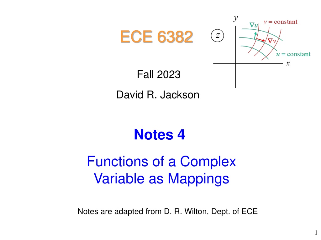
ECE 6382 Fall 2023 David R. Jackson Notes 4 Functions of a Complex Variable as Mappings Notes are adapted from D. R. Wilton, Dept. of ECE 1
A Function of a Complex Variable as a Mapping ( ) f z = A function of a complex variable, as a from the complex plane to the complex plane. mapping , is usually viewed w z w z w v y ( ) f z = w w = + w u iv = + x x iy z x u 3 = For example, w z 2
Simple Mappings: Translations Translation: where = is a complex constant. + w A z A z w y v = + w A z w z z x u A The mapping translates every point in the plane by the "vector" z A . 3
Simple Mappings: Rotations Rotation: ( ) ( ) + i i i i = = = w e z e re re real where is a constant. z w y v i = w e z z z x u w The mapping rotates every point in the plane through an angle z . 4
Simple Mappings: Dilations Note: ax, v du dv = Dilation (stretching): = = u ay ( ) i i = = = ( ) w az a re ar e = adx ady real where is a constant. a (All distances are uniformly stretched.) z y w v w = w z a z x u The mapping magnifies the magnitude in the complex plane by a facto of a point z z r . a 5
A General Linear Transformation (Mapping) is a Combination of Translation, Rotation, and Dilation Linear transformation: rotation dilation ( ) + Arg i B i Arg i B A = + = + = + w A Bz A B e r e B r e translation where are complex constants . A , B z y v w = + w A Bz B z z Arg B x u A w Shapes do not change under a linear transformation! 6
Simple Mappings: Inversions Inversion: 1 z 1 1 r i The magnitude becomes the reciprocal, and the phase angle becomes the negative. = = = w e i re Im x iy = + z r 1 Re = 1 w / z Points outside the unit circle get mapped to the inside of the unit circle. Points inside the unit circle get mapped to the outside of the unit circle. 7
Simple Mappings: Inversions Inversion: 1 z 1 1 r i = = = w e i re Im Im z = + z x iy 0 1 Re 1 Re 1 z 0x 1 z Inversion: circle-preserving property Inverson: a straight line maps to a circle Inversions have a circle preserving property, i.e., circles always map to circles (Straight lines are a special case where the radius of the circle is infinity.) 8
Circle Property of Inversion Mapping: Proof 1 z = w (This maps circles into circles.) + 1 w 1 + u + v = + = = = z x iy x , y 2 2 2 2 u iv u v u v ( ) ( ) 2 2 2 + = x x y y a Consider a circle: 0 0 2 2 2 2 a a x y + + + + = 0 x y a x a y a This is in the form 1 0 1 2 3 2 0 2 0 2 0 2 + a x y a 3 Hence 2 2 + + u + v u + v + + + + = 0 a a a 1 2 3 2 2 2 2 2 2 2 2 u v u v u v u v J. W. Brown and R. V. Churchill, Complex Variables and Applications, 9th Ed., McGraw-Hill, 2013. 9
Circle Property of Inversion Mapping: Proof (cont.) 2 2 + + u + v u + v + + + + = 0 a a a 1 2 3 2 2 2 2 2 2 2 2 u v u v u v u v Multiply by u2 + v2: 2 2 ( ) u + v + ( ) ( ) 2 2 + + + + + = 0 a u a v a u v 1 2 3 2 2 2 2 u v u v or ( ) ( ) ( ) 2 2 + + + + = 1 0 a u a v a u v 1 2 3 This is in the form of a circle (see next slide). 10
Circle Property of Inversion Mapping: Proof (cont.) ( ) ( ) ( ) 2 2 + + + + = 1 0 a u a v a u v 1 2 3 Divide by a3: 1 a a a a / a a / a ( ) 1 3 ( ) ( ) 2 2 1 2 0 + + + + = 0 u v a u a v a 2 2 / a 3 1 0 3 Complete the square: 2 2 a a ( ) ( ) 2 2 1 2 0 1 4 2 4 + + v a / + = 2 2 0 u a / a This is in the form of a circle: 1 + 2 2 u v a / a / 0 ( ) ( ) 2 2 2 u u + v v = R 0 2 2 0 0 2 a a 2 0 1 4 2 4 + R a ( ) 2 0 2 0 2 0 2 0 2 + + x y x y a 2 0 2 0 2 1 a 2 2 2 + x y 1 a 1 y a a a 2 = + = = = R ( ) ( ) ( ) 2 3 2 3 2 2 0 2 0 2 2 2 + 4 4 a x a 2 0 2 0 2 2 0 2 0 2 2 0 2 0 2 + + + x y a x y a x y a 3 11
Simple Mappings: Inversions (cont.) 1 z 1 1 r i = = = Geometrical construction of the inversion: w e i re w v u z w v y 1 z z = w z w 1 x u w Shapes are not preserved! Note the circular boundaries for the region! 12
Bilinear (a.k.a. Fractional or Mobius) Transformation + A Bz C + = w (A, B, C, D are complex constants) Dz Note that if 0 D , ( ) A BC D + + + B D C Dz + Dz A Bz C + A BC D C + = = = + w B D Dz C Dz Steps in : z w 1 A BC D C + A BC D C + + + z C Dz B D + C Dz Dz Dz This is a sequence of : linear transformation; inversion; dilation and rotation; translation. Since each transformation preserves circles, bilinear transformations also have the circle-preserving w the plane (with straight lines thought of as circles of infinite radius). property: circles in the plane are mapped into circles in z 13
Bilinear Transformation Example: The Smith Chart ( ) Z Z d ( ) ( ) ( ) = + = = + = Let where is the impedance at on a z r jx Z d R d jX d z -d 0 ( ) d transmission line of characteristic impedance reflection coefficient: and is the generalized Z , 0 ( ) ( ) ( ) ( ) z d + + + 1 1 Z d Z d Z Z z d 1 1 z z ( ) d 0 = = = or sim ly p 0 r x R / Z X / Z 0 Im x 0 + 1 1 z z = z r Re Normalized impedance plane Reflection coefficient plane Horizontal and vertical ines (contant reactance and resistance) are mapped into circles. For an interpretation of M bius transformations as projections on a sphere, see http://www.youtube.com/watch?v=JX3VmDgiFnY. 14
The Squaring Transformation ( ) w f z = = 2 2 2 i = z r e ( ) z, z w y v z w z w u x z 0 half entire The transformation maps The entire -plane covers the The transformation is said to be the -plane into the -plane twice. two-to-one. -plane. z w z w 15
Another Representation of the Squaring Transformation ( ) f z 2 2 2 i = = = w z r e 2 z y 180o 90o 3 270o 9 2 4 1 1 360o -360o x 0o 1 2 3 3D plot of magnitude -90o -270o -180o ( ) f z 2 = = Constant amplitude and phase contours of w z 16
The Square Root Transformation + 2 k p i i ( ) f z 1 2 / z = = = = = 0 1 , w re re , k 2 2 p v Note: The value of z1/2 on one branch is the negative of the value on the other branch. y z w z w Second branch u x w 0 2 = 1 k Principal branch = Re 0 0 k We say that there are two branches (i.e., values) of the square root function. Note that for the principal branch, the square root function is not continuous on the negative real axis. (There is a branch cut there.) The transformation is said to be one-to-two 17
The Square Root Transformation (cont.) + 2 k p i i ( ) f z 1 2 / z = = = = = 0 1 , w re re , k 2 2 p y The principal branch is the choice in MATLAB and most programming languages! v z w z w x u Principal branch = Re 0 0 k 1 1 = = 1 i + z The principal square root is denoted as 1 i = i 2 z 1 i Re 0 Note: = i 2 18
The Square Root Transformation (cont.) + 2 k p i i ( ) f z 1 2 / z = = = = = 0 1 , w re re , k 2 2 p y y 225o 45o 22.5o 202.5o 3 3 67.5o 247.5o 3 3 2 2 2 2 1 1 1 1 90o -90o 270o 90o x x 0o 180o 1 1 2 3 2 3 -22.5o -67.5o 157.5o 112.5o -45o 135o Principal branch, k = 0 Other branch, k = 1 19
Constant u and v Contours are Orthogonal ( ) ( ) Consider contours in the plane on which the real quantities are constant. y z v and z u x,y v x,y v = constant u ( ) ( ) ( ) = + = (analytic) w u x,y iv x,y f z u = constant x The directions normal to these contours are along the gradient direction: u x v x u y v y = + x y u = + x y v T he gradients, and therefore the contours, are orthogonal (perpendicular) by the C. R. conditions: C.R. cond's u x u y v x v y u x u y u y u x u y x u u u y x = + + = + + = + = x y x y x y x y 0 u v 20
Constant u and v Contours are Orthogonal (cont.) 2 = w z Example: ( ) ( ) ( ) 2 2 2 = + = + 2 w x iy x y i xy ( ( ) ) 2 2 = = u x,y x y so 2 v x,y xy Also, recall that ( ( v x,y y = = constant: v xy c ) ) 2 2 = 0 u x,y 2 = 0 2 2 = = constant: u x y c 1 x 21
Mappings of Analytic Functions are Conformal (Angle-Preserving) Consider a pair of intersecting paths , in the plane mapped C C z 1 2 = + onto the plane. w u iv y v ( ) f z = w w z ( ) z 1 2z w 0 f 1z 1 w 0 0z 0 C 1 w 2 2 C x 2 u ( ( ) ( ) ( ) ( ) z ( ) ( ) z + alo ng from arg arg arg w f z z w f z z , z C z 1 0 1 1 0 1 1 1 0 ) ) ( ) ( + a o g l n from arg arg arg w f z w f ( z , z C z 2 0 2 2 0 2 ) 2 2 0 ( ) ) ( arg arg arg arg w w z z 2 1 2 1 = Hence This assumes that f is not zero. 22
Constant u and v Contours are Orthogonal (Revisited) y v v = constant z ( ) f z w = w u = constant u x Since the contours u = constantand v = constant are (obviously) orthogonal in the w plane, they must remain orthogonal in the z plane. dz dw 0 Assumption: 23
Constant |w| and arg(w) Contours are also Orthogonal i = If the constant and contours are (obviously) orthogonal in the plane. w Re R w ( ) w 1 = If is a mapping back to the plane, the mapping preserves the orthogonality. z f z Note: dz dw 0 Assumption: The constant (red) and constant R (green) curves are obviously orthogonal in the w plane. y v = constant w z R = constant u x 24
The Logarithm Function ( ) z = ln w ( ) i + 2 k i = = p z z e z e ( ) ( ) z = + + k , k = 0 1 2 , ln ln 2 z i , , p There are an infinite number of branches (values) for the ln function! 25
Arbitrary Powers of Complex Numbers a = w z (a may be complex) Use ( ) i + 2 k ln z i = = = p z e z z e z e ) ( ( ) z ai + + ln 2 a k a ln a z ln ln a z a z ia 2 i ak p = = = = p z e e e e e e This has an infinite number of branches unless ak =integer for some value of k = q, i.e, a is real and rational: p q ( ) = a p,q are integers (In this case there are q branches.) 26
Arbitrary Powers of Complex Numbers (cont.) 2 3 / ( ) f z ( ) = = Example: 2 3 / z a Recall: ( ) i + 2 k 2 3 2 3 2 3 = p z z e ln z 2 i k i 2 3 / p = z e e e ln a z a ia 2 i ak = p z e e e 2 3 2 3 ln z 2 3 i 2 3 / p = = = 0 0 k k z e e 2 3 2 3 2 3 ( ) ln z 2 3 2 3 2 i i 2 3 / p = = = 1 k k z e e e 2 3 2 3 4 3 ( ) ln z 2 3 4 3 2 i i 2 3 / p = = = 2 k k z e e e 2 3 2 3 2 3 2 3 star r ts a ln ln z z 2 3 i i ( ) 2 3 / p p 2 2 i = = = = 3 2 k k z e e e e e e e t p i n g ! 2 3 8 3 2 3 = = = + r e p e a t s! 4 2 k k For zp/qthe repetition period is k = q (ifpand qhave no common factors). For irrational powers, the repetition period is infinite; i.e., values never repeat! 27


 is a")


")
")
")
 Transformation")


")
")

")


 Contours are also Orthogonal")


")