Understanding Cylindrical Wave Functions and Bessel Equations in Electromagnetics

Exploring cylindrical wave functions and Bessel equations, derived from the Helmholz equation, for understanding wave propagation dynamics in electromagnetics. The notes cover separation of variables, solutions for R and Z, Bessel functions, and more.

Understanding Cylindrical Wave Functions and Bessel Equations in Electromagnetics
PowerPoint presentation about 'Understanding Cylindrical Wave Functions and Bessel Equations in Electromagnetics'. This presentation describes the topic on Exploring cylindrical wave functions and Bessel equations, derived from the Helmholz equation, for understanding wave propagation dynamics in electromagnetics. The notes cover separation of variables, solutions for R and Z, Bessel functions, and more.. Download this presentation absolutely free.
Presentation Transcript
ECE 6382 Fall 2023 David R. Jackson Notes 20 Bessel Functions Notes are from D. R. Wilton, Dept. of ECE 1
Cylindrical Wave Functions Helmholtz equation: 2 + 2 = 0 k In cylindrical coordinates: 2 2 2 1 1 + + + + 2 = 0 k 2 2 2 2 z Separation of variables: ( ) ( ) = ( ) ( ) Z z , , z R let Substitute into previous equation and divide by . 2
Cylindrical Wave Functions (cont.) 2 2 2 1 1 + + + + 2 = 0 k 2 2 2 2 z ( ) ( ) = ( ) ( ) Z z , , z R 2 2 2 1 1 d R d dR d d d d Z dz + + + + = 2 0 Z Z RZ R k R Z 2 2 2 2 Divide by let 1 1 R R R R Z Z + + + + = 2 0 k 2 3
Cylindrical Wave Functions (cont.) 1 1 R R R R Z Z + + + + = 2 (1) 0 k 2 Therefore 1 1 Z Z R R R R = 2 k 2 ( , ) g ( ) f z Hence, ( ) f z = 2 z k constant 4
Cylindrical Wave Functions (cont.) Hence = Z Z 2 z k = = ik z ( ) ( ) ,sin( ),cos( ) Z z h k z e k z k z z z z z Next, to isolate the -dependent term, multiply Eq. (1) by 2: 1 1 R R R R + + + = 2 2 z 2 2 0 k k 2 5
Cylindrical Wave Functions (cont.) Hence 1 R R R R = + 2 2 2 z k k (2) ( ) g ( ) f Note: Hence If is allowed to change by 2 , then must be an integer. = 2 constant so i = = ( ) ,sin( ),cos( ) h e 6
Cylindrical Wave Functions (cont.) From Eq. (2) we then have 1 R R R R = + 2 2 2 2 z k k The next goal is to solve this equation for R( ). First, multiply by R and collect terms: ( ) + + = 2 2 2 2 z 2 0 R R k k R R 7
Cylindrical Wave Functions (cont.) 2 2 2 k k k Define z ( ) 2 + + = 2 2 0 R R k R Then, = = x k Next, define ( ) ( ) y x R dR d dy dx dx d ( ) ( ) = = = R y x k Note that ( ) p ( ) = 2 R y x k and 8
Cylindrical Wave Functions (cont.) + + = 2 2 2 0 x y xy x y Then we have Bessel equation of order ( ), x Y x ( ) J Two independent solutions: Hence = + ( ) y x ( ) x ( ) AJ BY x Therefore ( ) = ( ), ( ) R J k Y k 9
Cylindrical Wave Functions (cont.) Summary 2 + 2 = 0 k ( ) ( ) = ( ) ( ) Z z , , z R = ik z ( ) , sin( ), cos( ) Z z e k z k z z z z i = ), cos( , sin( ) e ( ) = ( ), ( ) R J k Y k + = 2 2 z 2 k k k 10
References for Bessel Functions M. R. Spiegel, Schaum s Outline Mathematical Handbook, McGraw-Hill, 4th Edition, 2012. M. Abramowitz and I. E. Stegun, Handbook of Mathematical Functions with Formulas, Graphs, and Mathematical Tables, National Bureau of Standards, Government Printing Office, Tenth Printing, 1972. NIST online Digital Library of Mathematical Functions (http://dlmf.nist.gov). N. N. Lebedev, Special Functions & Their Applications, Dover Publications, New York, 1972. G. N. Watson, A Treatise on the Theory of Bessel Functions (2nd Ed.), Cambridge University Press, 1995. 11
Plot of Bessel Functions 1 1 (0) J n =0 is finite 0.8 n =1 0.6 0 n =2 0.4 J0 x ( ) Jn (x) J1 x ( ) 0.2 Jn 2 x ( ) 0 0.2 0.4 0.403 0.6 0 1 2 3 4 5 6 7 8 9 10 0 xx 10 ( ) Note: 00 0. J 12
Plot of Bessel Functions (cont.) 1 0.521 n =0 0 n =1 1 n =2 2 Yn (x) Y0 x ( ) (0) Y is infinite Y1 x ( ) 3 Yn 2 x ( ) 4 5 6 6.206 7 0 1 2 3 4 5 6 7 8 9 10 0 xx 10 ( ) Note: 00 Y tends to infinity slower than the rest. 13
Frobenius Solution Frobenius solution*: ( ( ) k + 2 k 1 + x = ( ) x J ) ! ! 2 k k = 0 k ( ) = + ! 1 z z This series always converges. ( ) z = is analytic (has aTaylorseries) for Note: ( ). J n integer * The Frobenius series is a generalized Taylor series that has a non-integer set of powers. 14
Non-Integer Order n Non-integer order: = ( ) y x ( ), x J ( ) x J These are two valid solutions. Bessel equation is unchanged by Note: ( ) x J is always a valid solution These are linearly independent when is not an integer: ( ) x , ( ) x 0 J Ax J A x x as 1 2 15
Non-Integer Order (cont.) Bessel function of second kind: ( )cos( x ) ( ) x J J ( ) Y x sin( ) -2, -1, 0, 1, 2 This definition gives the Y (x)function a nice (simple) asymptotic form for large x. 16
Integer Order = n Integer order: ( ) lim ( ) Y x Y x n n ( )cos( J x ) ( ) x J ( ) Y x sin( ) 17
Integer Order (cont.) From the Frobenius solution we have: Notice the branch point at z = 0. ( ) k n 2 n k 1 ! 2 1 1 n x x ( ) x = + ( ) ln Y x J n n 2 ! 2 k = 0 k k n + 2 1 1 x ( ) ( ) k ( ) k + + 1 n k ( ) + ! ! 2 k n k = 0 k (Schaum s Outline Mathematical Handbook, Eq. (24.9)) where 0.577216 (Euler s constant) 1 2 1 3 1 p ( ) p ( ) 0 = + + + + = 1 ( 0), 0 p 18
Integer Order (cont.) Symmetry property: ( 1) = n ( ) x ( ) J J x n n ( 1) = n ( ) x ( ) Y Y x n n The functions J and J- are no longer linearly independent when is an integer. 19
Properties for General Orders Properties for General Orders In the following discussion, the order can be an integer or a non-integer value, as indicated. = integer n = arbitrary (with restrictions as indicated) 20
Small-Argument Formulas Small-Argument Properties (x 0): ( ) = n ( ) , 0,1,2 J x Ax n ( 1) = n ( ) x ( ) J J x n n n ( ) ( ) x , 1, 2, 3,... J Ax = ( 1) = n : ( ) x ( ) n J J x n n ( ) , Examples: ( ) ln Y x C x 0 1/ 2 1! 2 ( ) x J x ( ) x 1 x J x J = 1/2 n ( ) 1,2,3 Y x Dx n 0 n ( ) ( ) 1 / 2 1 ( ) , 0 Y x Bx / 2 J x x 1 2 1! 2 ( ) x J 1/2 x For order zero, the Bessel function of the second kind behaves logarithmically rather than algebraically. 21
Asymptotic Formulas Asymptotic Formulas: x 2 ( ) ~ x cos J x 2 4 x 2 ( ) ~ Y x sin x 2 4 x 22
Hankel Functions ( ) 1 + ( ) x ( ) x ( ) H J iY x ( ) 2 ( ) x ( ) x ( ) H J iY x x As 2 + ( ) i x Incoming wave* ( ) 1 ( ) ~ x H e 2 4 x 2 ( ) i x ( ) 2 Outgoing wave* ( ) ~ x H e 2 4 x ( ) ( ) + i t * assuming time convention exp These are valid for arbitrary order . 23
Hankel Functions (cont.) y Useful identity: z x ( ) ( ) 2 n ( ) 1 n + 1 n = + ( ) 1 ( ) H z H z z ( ) z Im 0 This is a symmetry property of the Hankel function. N. N. Lebedev, Special Functions & Their Applications, Dover Publications, New York, 1972. 24
Generating Function The integer order Bessel function of the first kind can also be defined through a generating function g(x,t): 1 t xt = ( ) ( ) x t n 2 , g x t e J (derivation omitted) n = n The generating function definition leads to various useful identities and representations: ( ) ( ) n in ikx = e i J k e (plane wave expansion, a.k.a.Jacobi- Anger expansion) n = n 1 ( ) x ( ) = cos sin J x m d (integral representation of Bessel function) m 0 (Please see next slides.) 25
Generating Function (cont.) Plane-wave expansion: 1 t ) ( k t i i ie ie 2 ( ) ( ) ik ik ikx cos cos = = = = 2 e e e e e = = , k ie i t Hence, using the generating function identity, we have: = ( ) ikx n e J t n = = , k ie = n i t so ( ) ( ) n in ikx = e i J k e n = n 26
Generating Function (cont.) The plane wave expansion is very useful for solving scattering problems in cylindrical coordinates: ( ) ( ) jkx jn n (using j instead of i) = e j J k e n = n y Cylinder Plane wave a x Top view of scattering of a cylinder by a plane wave 27
Example Example: Acoustic plane-wave scattering by a cylinder. (x, y, z) = acoustic pressure function ( ) ( ) ( ) jkx jn n = = (using j instead of i) inc , , x y z e j J k e n = ) = n ( )( n ) ( ( ) jn n 2 sca , , x y z j a H k e Assume: n = n Acoustic hard cylinder: = ( ) ( ) ( ) = + inc sca , , x y z , , x y z , , x y z ( ) = 0 a y n 2 Cylinder = = k Plane wave c a 0 0 x 0c = speed of acoustic wave 28
Example (cont.) ( ) ( ) ( ) jn n = inc , , x y z j J k e n = n ( ) = = = 0 a ( )( n ) n ( ) ( ) jn n 2 = sca , , x y z j a H k e n = n ( )( n ) ( ) ( ) ( ) jn jn n n n 2 = j k J ka e j a k H k a e n = = n n ( ) n J ka k a = a ( )( n ) n 2 H 29
Generating Function (cont.) Integral representation of Bessel function: ( ) ( ) cos ik in n Start with: = e i J k e n = n = im Set Integrate over in above result, multiply both sides by , use orthogonality f 1 k e Orthogonality: = ( ) 2 2 , 0, m n in o 0,2 e ( ) i m n = e d m n 0 2 m ( ) ( ) cos i im = 2 e e d i J m 0 m 2 i ( ) cos i im = J e e d m 2 0 30
Generating Function (cont.) Integral representation of Bessel function (cont.): m 2 i ( ) cos i im = J e e d m 2 0 = + Use symmetry, : / 2, m 2 /2 i ( ) ( ) + + cos /2 /2 i im ( ) = J e e d m 2 /2 m 2 /2 i ( ) + sin i ( ) im m = e e i d 2 /2 2 1 ( ) + sin i im = Periodic integrand e e d 2 0 31
Generating Function (cont.) Integral representation of Bessel function (cont.): 2 1 ( ) + sin i ( ) im = J e e d m 2 0 1 ( ) + sin i im = e e d 2 1 ( ) ( ) = + cos sin sin sin m i m d 2 1 ( ) cos sin m d 2 odd function 1 ( ) = cos sin m d 0 1 ( ) x ( ) = cos sin J x m d ( is relabeled as x) m 0 32
Recurrence Relations Many recurrence relations can be derived from the generating function. 1 t xt ( ) = = n 2 , ( ) x t g x t e J n = n 1 t xt = 1 n 2 ( ) x t e nJ n t = n 1 t xt 1 t x + = 1 n 2 1 ( ) x t e nJ n 2 2 = n 1 t x + = 1 n n 1 ( ) x t ( ) x t J nJ n n 2 2 = = n n x ( ) + = 2 1 n n n ( ) x t ( ) x t J t nJ n n 2 = = n n + On LHS use: 1 & 1 n n n n x + = 1 1 n n ( ) x ( ) x t ( ) x t J J nJ + 1 1 n n n 2 = = n n 33
Recurrence Relations (cont.) x + = 1 1 n n ( ) x ( ) x t ( ) x t J J nJ + 1 1 n n n 2 = = n n Equating like powers of t yields: 2 n x + = ( ) x ( ) x ( ) x J J J + 1 1 n n n 34
Recurrence Relations (cont.) 2 n x + = ( ) x ( ) x ( ) x J J J + 1 1 n n n This can then be used to generate other useful recurrence relations: ( ) 2 1 n = ("upward recursion") 1: ( ) x ( ) x ( ) x n n J J J 1 2 n n n x + ( ) 2 1 n + = ("downward recursion") 1: ( ) x ( ) x ( ) x n n J J J + + 1 2 n n n x 35
Recurrence Relations (cont.) Another recurrence relation for the derivative of the Bessel function: 1 t xt = ( ) = n 2 , ( ) g x t e J x t n = n For the LHS: 1 t xt 1 t x 2 1 2 1 t 1 2 1 t e t ( ) = = = n 2 , ( ) g x t t e t J x t n x x = n 1 2 + = 1 1 n n ( ) ( ) J x t J x t n n = = n n 1 2 1 2 = = n n n ( ) x t ( ) x t ( ) x ( ) x t J J J J + + 1 1 1 1 n n n n = = = n n n Also, we have, for the RHS: ( ) n = n , ( ) x t g x t J x = n 1 2 n = ( ) x ( ) x ( ) x J J J Equating like powers of t yields: + 1 1 n n 36
Recurrence Relations (cont.) 1 2 n = ( ) x ( ) x ( ) x J J J + 1 1 n n Then use the previous identity: 2 n x + = ( ) x ( ) x ( ) x J J J + 1 1 n n n This can be used to replace Jn+1 or Jn-1. This yields: n x n = ( ) x ( ) x ( ) x J J J 1 n n n x n = + ( ) x ( ) x ( ) x J J J + 1 n n 37
Recurrence Relations (cont.) The same recurrence formulas actually apply to all Bessel functions of all orders. If Z (x) denotes any Bessel, Neumann, or Hankel function of order , then we have: 2 + = ( ) x ( ) x ( ) Z Z Z x + 1 1 x ( ) 2 1 = ( ) ( ) x ( ) x Z x J J 1 2 x ( ) + 2 1 = ( ) ( ) x ( ) x Z x J J + + 1 2 x = = + Z Z Z Z Z Z + 1 1 x x 38
Recurrence Relations (cont.) Integral identities also follow from the recurrence identities. Example of integral identity: = + = Z Z Z xZ Z xZ (multiplying both sides by x) 1 1 x + = 1 1 Multiply by x x Z x Z x Z 1 Hence, d dx + = = 1 ( ) ( ) x x Z x Z x Z x x Z 1 = 1( ) x dx ( ) x Z x Z x Similarly, we have = 1( ) x dx + ( ) x Z x Z x 39
Recurrence Relations (cont.) Examples: ( ) x xdx ( ) x = J xJ (First one, = 1) 0 1 ( ) x dx ( ) x (Second one, = 0) = J J 1 0 40
Wronskians 2sin ( ) ( ) x J ( ) x ( ) x J ( ) x = = Please see the note below. , W x W J J J J x 2 ( ) x Y ( ) x ( ) x Y ( ) x = = , W J Y J J + (1) x H for 2 i x ( ) x H ( ) x ( ) x H ( ) x (2) H W J H = = for (1,2) (1,2) (1,2) , J J Note: For n, the Wronskian is [J ,J- ] is not identically zero (in fact, it is not zero anywhere), and hence the two functions are linearly independent. (Please see Appendix A for a derivation.) 41
Fourier-Bessel Series Fourier-Bessel series: Note: The order and the length a are arbitrary here. ( ) = , 0 f c J p a n n a = 1 n = th where is the zero o f ( ): x ( ) 0. p n J J p n n The coefficients are given by a 2 = ( ) c f J p d ( ) n n 2 2 a J p a + 1 n 0 (Please see Appendix B for a derivation.) 42
Addition Theorems y Addition theorems allow cylindrical harmonics in one coordinate system to be expanded in terms of those of a shifted coordinate system. y x 0 0 x 0 Shifting from global origin to local origin: ( ) i n m = in im ( ) ( ) ( ) J k e J k e J k e 0 n m 0 n m = m ( ) i n m (2) n m im ( ) ( ) , H k e J k e 0 0 0 m = m = (2) n in ( ) H k e ( ) i n m (2) m im ( ) ( ) , J k e H k e 0 n m 0 0 = m 43
Addition Theorems (cont.) y y x 0 0 0 x Shifting from local origin to global origin: )( ) ( i n m + = in im ( ) ( ) ( ) J k e J k e J k e 0 n m 0 n m = m )( ) ( i n m + (2) n m im ( ) ( ) , H k e J k e 0 0 0 m = m = (2) n in ( ) H k e )( ) ( i n m + (2) m im ( ) ( ) , J k e H k e 0 n m 0 0 = m 44
Addition Theorems (cont.) y y Recall: x ( ) x ( ) ( ) ( )( ) m m = 1 J J x 0 m m 0 ( )( ) m ( ) ) m 2 2 = 1 H x H x x 0 ( m = im 1 e Shifting from local origin to global origin: Special case (n = 0): ( ) = im ( ) ( ) ( ) J k J k J k e 0 0 0 m m = m ( ) im (2) m ( ) ( ) , H k J k e 0 0 0 m = = m (2) 0 ( ) H k ( ) im (2) m ( ) ( ) , J k H k e 0 0 0 m = m 45
Appendix A: Wronskians From the Sturm-Liouville properties, the Wronskians for the Bessel differential equation are found to have the following form: Recall: x dx x x x a a x ( ) x W a a C x ( ) p x dx + ln ln = = = = = ( ) ( ) ( ) ( ) W x W a e W a e W a e = ( ) ( ) W x W a e p x p x a a ( ) ( ) ( + 1 ( ) p x 0 ) The constant C can be found using the small-argument approximations for the Bessel functions (keep k = 0 term in the Frobenius series). The result is: + = 2 2 2 0 x y xy x y ( ) ( ) = = 2 p x x 0 p x x 1 2sin ( ) ( ) x J ( ) x ( ) x J ( ) x = = , W x W J J J J x (Please see next slide.) Note: For n, the Wronskian is not identically zero (in fact, it is not zero anywhere), and hence the two functions are linearly independent. 46
Appendix A (cont.) ( ( ) k + 2 k 1 + x = ( ) x J ) ! ! 2 k k = 0 k 1 1 x x ( ) x , ( ) x J J ( ) ! 2 ! 2 ( ( ) ) 1 1 1 2 ! 2 1 2 x x ( ) x ( ) x , J J ! 2 2 ( ) ( ) x J ( ) x ( ) x J ( ) x = = = W x J J ( ) ( ) ( ) ! ! ! ! ! ! x x x Recall: 2 2sin = = C ( ) ( ) (1 z = ) z ! ! sin z ( ) (1 = ) sin 2sin ( ) = W x ( ) ( 1 ! ) = ! x sin ( ) ( ) = ! ! sin 47
Appendix A (cont.) Similarly, we have 2 ( ) x Y ( ) x ( ) x Y ( ) x = = , W J Y J J x 2 i x ( ) x H ( ) x ( ) x H ( ) x W J H = = (1,2) (1,2) (1,2) , J J + (1) H for (2) H for 48
Appendix B: Fourier-Bessel Series To derive the Fourier-Bessel expansion, start with: ( ) = , 0 f c J p a n n a = 1 n Multiply both sides by and integrate from 0 to a: m J p a a a ( ) = f J p d c J p J p d m n n m a a a = 1 n 0 0 a = c J p J p d n n m a a 10 = n 2 a ( ) (using orthogonality + result from next slide) = 2 c J p + 1 m m 2 Note: See Notes 18 for a derivation of the orthogonality when m n. 49
Appendix B (cont.) Derivation of the orthogonality formula Start with this integral identity (derivation omitted): 2 2 2 x x ( ) ( ) ( ) ( ) ( ) 2 2 = 2 1 J px xdx J px J px ( ) 2 2 2 px = / Choose : p p a m 2 2 a 2 2 2 p p p a a = 2 1 m m m J x xdx J a J a 2 2 2 a a a p 0 a m a 2 a ( ) ( ) 2 = J p m 2 Recall: 2 2 a = + ( ) ( ) J p J p + ( ) x 1 m m = + ( ) x ( ) x J J J 2 p + 1 m x 2 a ( ) 2 = ( ) J p + 1 m 2 50


")
")
")
")
")
")
")
")


")


")

")
")


")

")
")

")
")
")
")

")
")
")
")
")
")
")


")
")

")
")

")