Visualizing Mathematical Functions with Matplotlib
Download Presenatation

Discover how to create visually appealing plots of mathematical functions using Matplotlib in Python. From simple sine and cosine curves to more complex exponential functions, learn step-by-step how to generate and customize plots for various mathematical expressions.

Download Presentation
Please find below an Image/Link to download the presentation.
The content on the website is provided AS IS for your information and personal use only. It may not be sold, licensed, or shared on other websites without obtaining consent from the author. If you encounter any issues during the download, it is possible that the publisher has removed the file from their server.
You are allowed to download the files provided on this website for personal or commercial use, subject to the condition that they are used lawfully. All files are the property of their respective owners.
The content on the website is provided AS IS for your information and personal use only. It may not be sold, licensed, or shared on other websites without obtaining consent from the author.
E N D
Presentation Transcript
# [-2 , 2 ] >>> import numpy as np >>> import matplotlib as mpl >>> import matplotlib.pyplot as plt >>> x=np.linspace(-2*np.pi, 2*np.pi,100) >>> y=np.sin(x) >>> plt.plot(x,y) >>> plt.show()
>>> import numpy as np >>> import matplotlib as mpl >>> import matplotlib.pyplot as plt >>> x=np.linspace(-2*np.pi, 2*np.pi,100) >>> y=np.sin(x) >>> y1=np.cos(x) >>> fig=plt.figure(figsize=(6,3), facecolor= 0.8 ) >>> fig.suptitle( , [-2 ,2 ] , fontsize=12) >>> ax=fig.add_axes((0.1,0.1,0.8,0.8), facecolor= 0.95 ) >>> ax.plot(x,y, g: , linewidth=3) >>> ax.plot(x,y1, r ,linewidth=2) >>> plt.show()
import numpy as np import matplotlib as mpl import matplotlib.pyplot as plt x=np.linspace(-2*np.pi, 2*np.pi,40) y=np.sin(x) y1=np.cos(x) fig, axs=plt.subplots(nrows=2, ncols=1, figsize=(8,5)) fig.tight_layout(pad=1.5) axs[0].set_facecolor('0.95') axs[1].set_facecolor('0.95') axs[0].plot(x,y,marker='o', markersize=8, markerfacecolor='#FFA500', markeredgewidth=1, markeredgecolor='xkcd:petrol') axs[1].plot(x,y1,'g*--',linewidth=2.0) plt.show()
import numpy as np import matplotlib as mpl import matplotlib.pyplot as plt t=np.linspace(0, 70,500) y=np.exp(-t/10)*np.cos(t) fig, axs=plt.subplots(figsize=(8,5)) axs.plot(t,y) axs.set_xlabel('t->secs', labelpad=6, fontsize=10, fontname='sans serif', style='italic') axs.set_ylabel('y=f(t)', labelpad=6, fontsize=10, fontname='serif') axs.set_title(' ', fontsize=14, fontname='monospace', color='green', loc='center', pad=7.0) plt.show() #y(t)=e^(-t/10)cos(t)